First, check the data headers of the data we are going to process. The actual data processing usually starts from editing the data headers. Fortunately, the header of the dataset here has already been finished editing. The headers contain the basic information of the dataset.
$ surange < Nshots.suThe output is as follows (it may take some minutes because the dataset is large.).
-----
19057 traces:                              : Number of traces
tracl    39069 58125 (39069 - 58125)       : Trace number
tracr    1 19057 (1 - 19057)               : Trace number
fldr     1687 2012 (1687 - 2012)           : Shot number
tracf    28 96 (96 - 28)                   : Receiver number
cdp      900 1300 (900 - 1300)             : CDP (CMP) number
cdpt     1 69 (1 - 1)
trid     1 2 (1 - 1)                       : Data type
offset   -2435 -170 (-170 - -2435)         : Offset distance (m)
scalel   -10000
scalco   -10000
counit   1
muts     0 11000 (0 - 0)
ns       5500                              : Number of samples in the trace
dt       2000                              : Sampling time (micro second)
day      206
hour     21 22 (21 - 22)
minute   0 59 (3 - 20)
sec      1 59 (45 - 3)
-----
The range of each header value is displayed.
Next, take a look at the data. Since the dataset is too large to display all, extract a portion of the dataset and display it.
For example, extract the traces whose shot number (in the header "fldr") is from 1800 to 1805, sort the data on the order of receiver number (in the header "tracf") and create a small subset of the data, such as "tmp_1800.su". The range of shot and receiver number and the name of the file are of your choice.
$ suwind key=fldr min=1800 max=1805 < Nshots.su > tmp.su
$ susort tracf < tmp.su > tmp_1800.su
$ rm tmp.su
Display some headers (here, "fldr", "tracf", "cdp", "offset").
$ surange < tmp_1800.su
$ sugethw key=fldr,tracf,cdp,offset < tmp_1800.su
Display the data.
$ suxwigb perc=98 < tmp_1800.su &
$ suximage perc=98 < tmp_1800.su &
This is a dataset of a marine survey. Therefore,
cdp 1 2869 (1 - 2869).This indicates that the dataset "Nshot.su" is a subset of a dataset that created "Nstack.su".
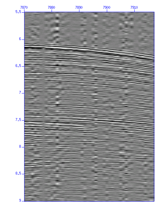
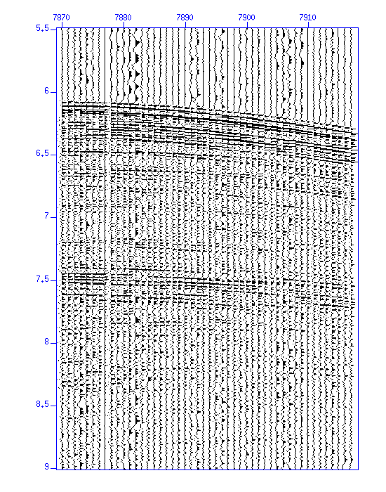
$ suwind key=cdp min=1095 max=1095 < Nshots.su > cdp_1095.suDisplay the waveforms.
$ suximage < cdp_1095.su perc=99 &
$ suxwigb < cdp_1095.su perc=99 &
Fig: Waveforms (enlarged) (Left) in an image, (Right) in wiggle traces.
$ suspecfx < cdp_1095.su | suximage perc=98 &
$ suspecfx < cdp_1095.su | suxgraph &
$ suspecfx < cdp_1095.su | suop op=db | suxgraph &
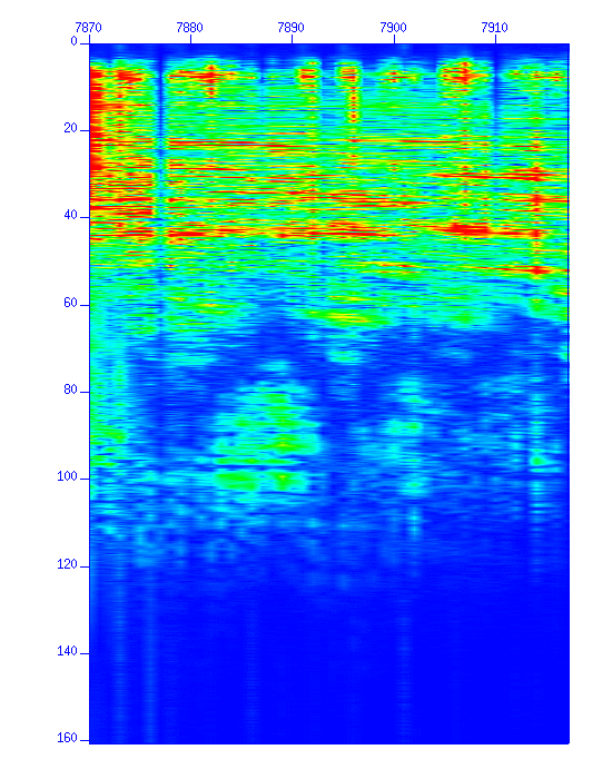
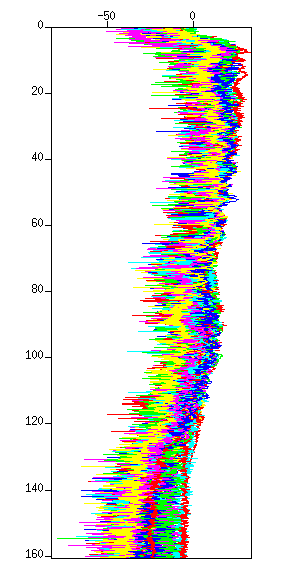
Fig: Spectrum. (Left) The spectrum in a color image. The vertical axis is "frequency (Hz)". (Right) The spectrum in a graph style.
Now you can see the frequency components contained in the data.
Then, check the components in each frequency band. A simple shell script, create_BPF_panel.sh displays the frequency components at every 10 Hz, each has a 10 Hz bandwidth (0-10, 10-20, ...) Edit the filename in the script so that the script can use your data file.
$ sh create_BPF_panel.sh
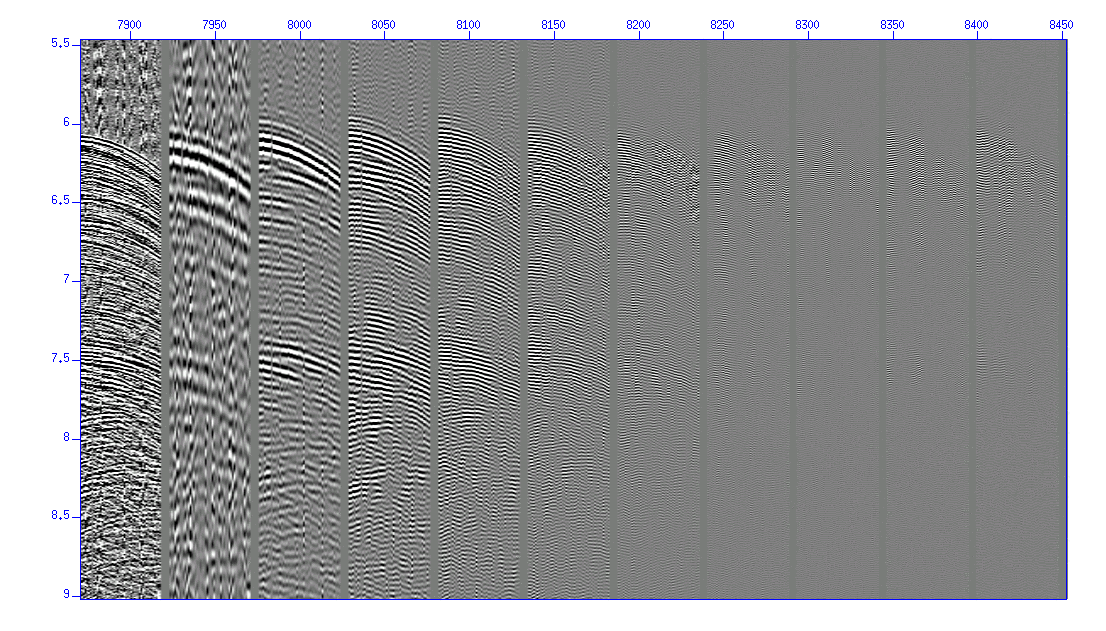
Fig: Spectrum, (Left) Original, (Rights) After band-pass filtering of 0-10, 10-20 Hz, 20-30Hz, 30-40Hz, ......
Try applying a band-pass filter to the sample data. The example below uses 'f=10,20,70,80'.
$ sufilter f=10,20,70,80 amps=0,1,1,0 < cdp_1095.su | suspecfx | suximage perc=98 &
$ sufilter f=10,20,70,80 amps=0,1,1,0 < cdp_1095.su | suspecfx | suxgraph &
$ sufilter f=10,20,70,80 amps=0,1,1,0 < cdp_1095.su | suspecfx | suop op=db | suxgraph &
$ sufilter f=10,20,70,80 amps=0,1,1,0 < cdp_1095.su | suximage perc=99&
You may want to eliminate or reduce the low and high frequency noise seen in the sea water (which should have no reflections). Try and find an appropriate filter paramenters and apply it to your sample data.
$ sufilter f=?,?,?,? amps=0,1,1,0 < cdp_1095.su > cdp_1095_flt.su
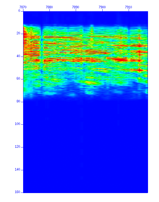
Fig: Spectrum in color display, (Left) the original, (Right) after band-pass filtering.
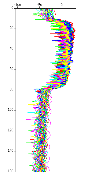
Fig: Spectrum in graph display, (Left) the original, (Right) after band-pass filtering.
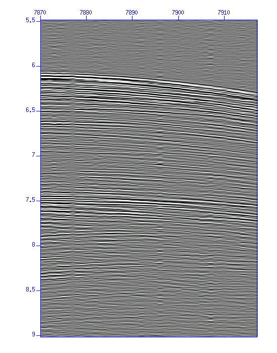
Fig: Waveforms in image display, (Left) the original, (Right) after band-pass filtering.
$ suximage perc=98 < cdp_1095f.su &
$ suop op=nop  < cdp_1095f.su | suattributes mode=amp | suop op=db |suxgraph &
$ sugain tpow=2.0 < cdp_1095_flt.su | suattributes mode=amp | suop op=db | suxgraph &
$ sugain tpow=? < cdp_1095_flt.su > cdp_1095_flt_gain.su
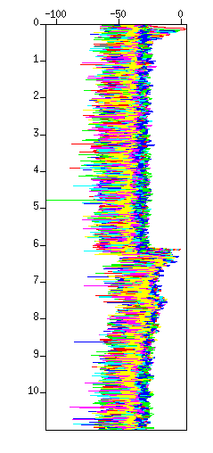
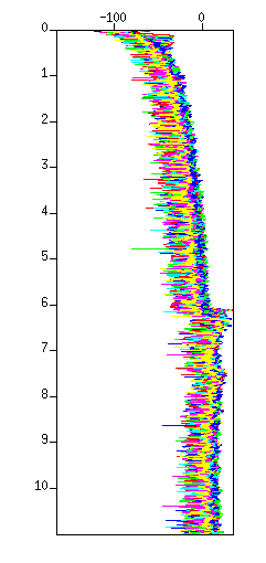
Fig: Waveforms in amplitude display, (Left) Before the amplitude recovery (after the filter), (Left) after the amplitude recovery. Note that the amplitude after 6.0 seconds became flat.
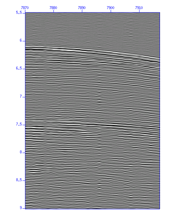
Fig: Waveforms in image display, (Left) Before the amplitude recovery (after filter), (Left) after the amplitude recovery. Note the amplitude of deeper reflections increased.
The f-k spectrum is displayed for your reference.
$ suspecfk < cdp_1095_fg.su | suximage perc=98 &
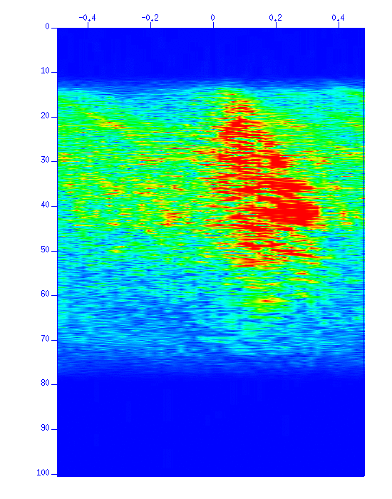
Fig: f-k spectrum.
As the velocity filter will be applied to each shot gather (common-shot record), you will need to use a shell script to loop the filtering operation through all shot gathers.
If you are interested in applying the deconvolution, visit here and follow the guidance. It is a good idea to compare the result with and without deconvolution.
This is the end of the parameter seeking for preprocessing. Keep the file you've created, for example, "cdp_1095_flt_gain.su" (if you applied the deconvolution, the file name should be "cdp_1095_flt_gain_decon.su" or whatever) since it will be used in the next exercise.
$ sufilter f=?,?,?,? amps=0,1,1,0 < Nshots.su | sugain tpow=? | suresamp nt=2750 dt=0.004 > Nres.suYou should use the values you've chosen in place of '?'.
If you are to apply deconvolution, the command line should be something like below.
$ sufilter f=?,?,?,? amps=0,1,1,0 < Nshots.su | sugain tpow=? | supef minlag=???? | sufilter f=?,?,?,? amps=0,1,1,0 | suresamp nt=2750 dt=0.004 > Nres.su
Finally, sort the data on the order of 'cdp', then sort on the order of 'offset' in each 'cdp'.
$ susort cdp offset < Nres.su > Ncdps.suThe preprocessing is now completed!
-rw-r--r-- 1 watanabe staffs 214200680 Nov  7 12:17 Ncdps.su
-rw-r--r-- 1 watanabe staffs 423827680 Nov  7 12:17 Nshots.su
The size of the new dataset is roughly half of the original. You can delete the intermediate data "Nres.su".