Geophysical Exploration of Crustal Structure

Exercise 7: Processing of real data

Processing flow

1. Check headers (Done)
2. Band-pass filter (Done)
3. Amplitude recovery (Done)
4. Velocity (f-k) filter (Optional)
5. Deconvolution (Optional)
6. Static corrections (Not mentioned)
7. Velocity analysis
8. NMO correction and CMP stacking
9. Migration

Velocity analysis

First, display a semblance panel of the Constant-Velocity-Stack (CVS).

$ suvelan nv=160 dv=25 fv=1000 < cdp_1095_flt_gain.su | suximage f2=1000 d2=25 perc=99 mpicks=pick.txt &

• "suvelan" creates a semblance panel (a panel containing amplitude information after NMO and stack) of the Constant-Velocity-Stack (CVS).
• 'nv=160 dv=25 fv=1000' indicates that the 160 velocity values starting from 1000 m/s with the interval of 25 m/s are to be used.
• For 'f2' and 'd2' in "suximage", use the value of 'fv' and 'dv' of "suvelan", respectively.
• Use the left-button of the mouse to zoom in to the area of interest.
• Clicking the mouse-middle-button picks the coordinate of the location of the mouse. Pressing 's' outputs the mouse location to a file.
• 'mpicks=' indicates the file that the picked values are to be stored.
• !Caution! Pick the values on the order as t (time) increases (downward).
• !Caution! Recall the picked velocity is a RMS average of the layer velocities. Therefore, avoid rapid velocity changes when picking because a rapid change in stacking velocity generates a very high (or low) velocity layer.
• !Caution! Be sure to press the key 'q' on the keyboard when you finish picking to close the "ximage" window. DO NOT close the window by clicking the close button using a mouse or you will lose your picking result.

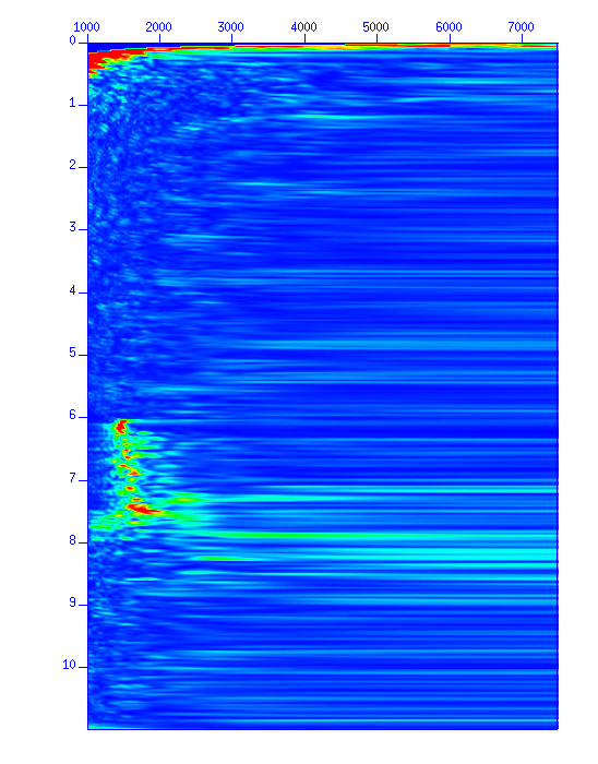
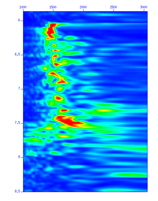
Fig: A CVS semblance panel. The vertical axis is "time (s)" and the horizontal axis is "velocity (m/s)" (Left) All, (b) a zoomed portion.

Then, reshape the format of the pick-file "pick.txt" so that the picked values can be used as the input of the NMO correction program.

$ mkparfile < pick.txt > pick.par string1=tnmo string2=vnmo

NMO correction and CMP stacking

sunmo par=pick.par < cdp_1095_flt_gain.su | suximage perc=98 &
sunmo par=pick.par < cdp_1095_flt_gain.su | suxwigb perc=98 &

If it looks OK, then apply CDP stacking. If you are not satisfied with the correction, go back to Velocity analysis and do it again.

sunmo par=pick.par < cdp_1095_flt_gain.su | sustack | suxwigb perc=98 &
sunmo par=pick.par < cdp_1095_flt_gain.su | sustack | suximage perc=98 &

Application to the dataset

You can modify the parameters at the beginning of the script. Instead, you can edit the parameters in a separate file, "parameters_for_interactive_velocity_analysis.par". If the file exists, the script reads the file. The parameters in the file has the priority.

$ emacs parameters_for_interactive_velocity_analysis.par &
$ vi parameters_for_interactive_velocity_analysis.par

#================================================
# USER AREA -- SUPPLY VALUES
#------------------------------------------------
# CMPs for analysis

# CMPs
cmp1=933
cmp2=958
cmp3=983
cmp4=1008
cmp5=1033
cmp6=1058
cmp7=1083
cmp8=1108
cmp9=1133
cmp10=1158
cmp11=1183
cmp12=1208
cmp13=1233
cmp14=1258
cmp15=1283

# Number of CMPs
numCMPs=15

#------------------------------------------------
# File names

indata=Ncdps.su      # SU format
outpicks=Nvpick.txt  # ASCII file

#------------------------------------------------
# display choices

myperc=95       # perc value for plot
plottype=1      # 0 = wiggle plot,  1 = image plot

percvelan=99    # perc value for Velocity Analysis Panel

# More parameters are customizable. See the script itself.
# end

• Write the CMP numbers you chose to apply velocity analysis from 'cmp1' in ascending order.
• Set the number of CMPs you chose as 'numCMPs='. Be sure to the number of 'cmp??=' and the value of the 'numCMPs=' are identical.
• The file names are of your choice.
• The script runs as it is. In this case, you will do velocity analysis at 15 CMP locations, which may be somewhat tough work.

Execute the shell script.

$ sh interactive_velocity_analysis.sh

• When starting the script, 3 windows named
  • "Semblance Plot",
  • "Constant Velocity Stacks",
  • "CMP gather"
  will open (from left to right). You have experienced these plots in the past exercises.
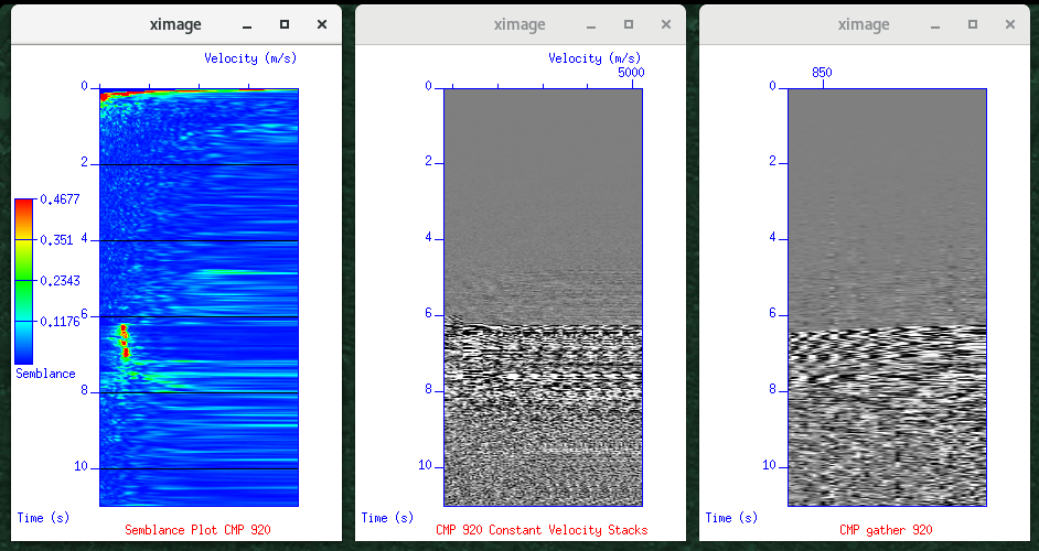
• To pick and read the velocity, the "Semblance Plot" on the left is used.
• Zoom the plot at the time from 5 to 8 seconds. Then, locate the mouse on the high semblance value (indicated in Red) and press 's' to read the value.
• Pick at least 4 or 5 (not too many) points as time increases.
• [Hint] The stacking velocity may range from 1500 to 2300 m/s. Avoid rapid changes in velocity.
• Press 'q' to close the window when you finish picking.
• Then, following new windows will come up.
  • CMP after NMO,
  • CMP repeat stack trace,
  • Stacking Velocity Function
  • Interval Velocity Function
  The above two shows the result of NMO and CMP stacking using the velocity structure you picked.
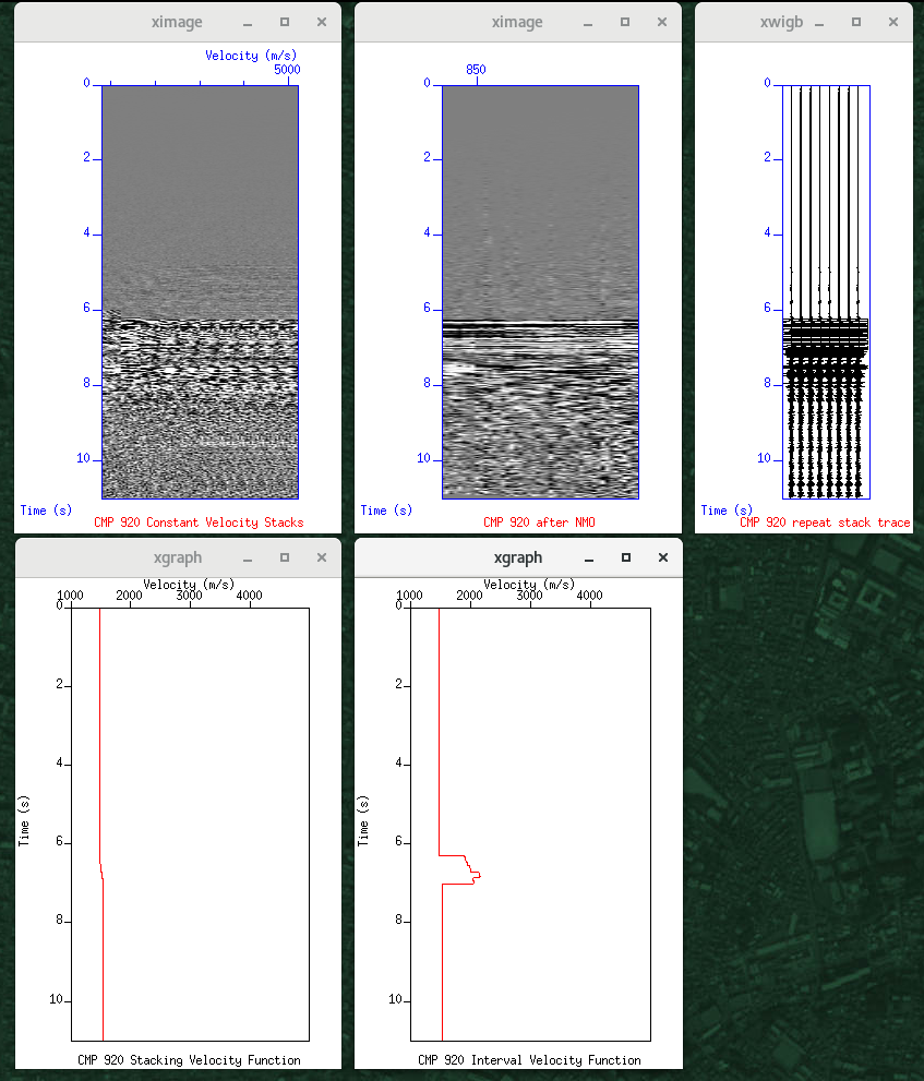
• "Stacking Velocity function" shows the velocity structure generated by your picking.
• "Interval Velocity function" shows the interval velocity derived from the stacking velocity using DIx's formula. If the interval velocity is too small or too large, you may want to try improving your velocity picking again.
• On the console (terminal) where you run "interactive_velocity_analysis.sh", you are to be asked if your pick is OK. Answer (y/n). "y" goes next. "n" returns picking.
• If you returned, your previous pick will appear for your reference.
• Repeat picking until you process all your CMPs.

$ cat Nvpick.txt

cdp=950,1050,1150,1200,1280 \
tnmo=0,6.20617,6.54153,6.85235,7.17952,7.51488,7.89113 \
vnmo=1500,1453.33,1488.89,1640,1648.89,1666.67,1915.56 \
tnmo=0,6.02364,6.59894,7.08253,7.39103,7.7162 \
vnmo=1500,1518.19,1669.86,1644.58,1631.94,1859.44 \
...

Execute the NMO correction and the CMP stacking using the picked result.

$ sunmo par=Nvpick.txt < Ncdps.su | sustack > Nzerooffset.su
$ suximage perc=98 < Nzerooffset.su &

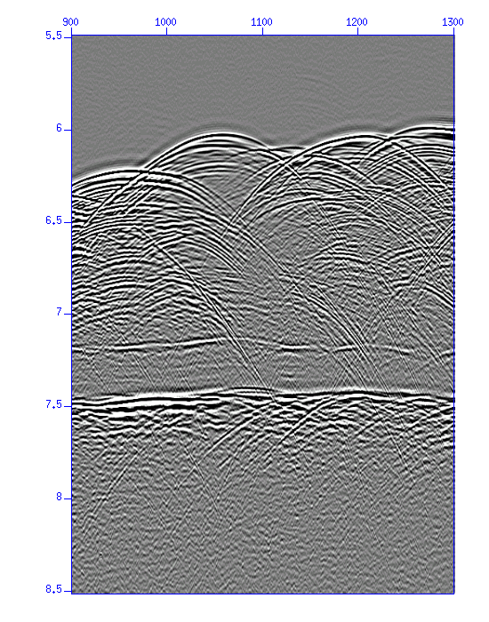
Fig: A zero-offset section by CMP stacking.

Displaying the velocity structure

This script required the result of the velocity analysis (Nvpick.txt). Display the velocity structure you created using the result of the velocity analysis. Both the stacking velocity and the interval velocity will be displayed.

$ sh plot_velocity.sh

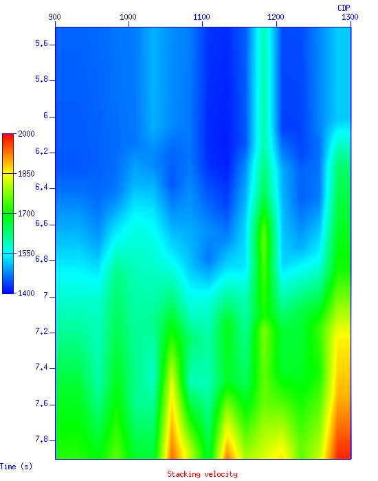
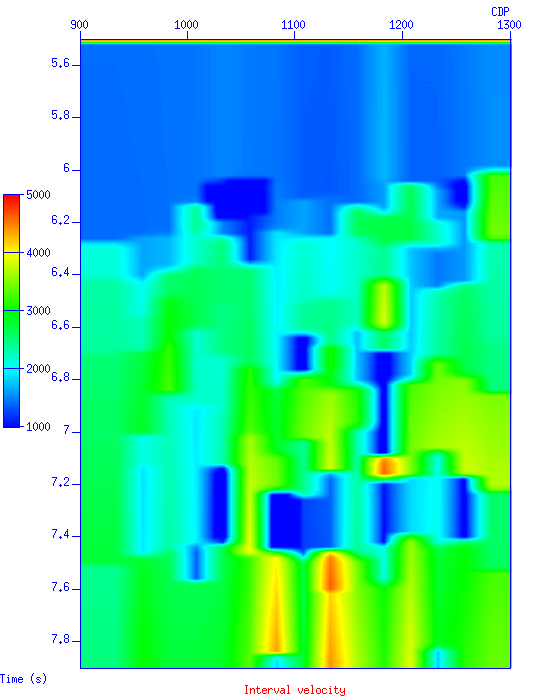
Fig: Velocity structure obtained by velocity analysis, (Left) Stacking velocity, (Right) Interval velocity.

Migration

We will use Stolt migration (Stolt, 1978), which is an extension of f-k migration, among a lot of migration algorithms. The major reason is its short computation time. First, start with a trial.

$ sustolt cdpmin=900 cdpmax=1300 dxcdp=16.667 vmig=1500 tmig=6 < Nzerooffset.su | suximage perc=98 &
$ sustolt cdpmin=900 cdpmax=1300 dxcdp=16.667 vmig=1500 tmig=6 lstaper=20 lbtaper=100 < Nzerooffset.su | suximage perc=98 &

• "sustolt" does time-migration proposed by Stolt (1978).
• 'cdpmin=900 cdpmax=1300' because CDP No. is from 900 to 1300.
• The CDP interval is 'dxcdp=16.667' (m).
• 'vmig=????' gives velocity (m/s). First, we use a constant velocity of 1500 (m/s).
• 'tmig= ' and 'vmig= ' are the pairs used to specify the velocity structure. In this case, as the velocity is constant, any value can be used, for example, 'tmig= 6' (s).
• 'lstaper' and 'lbtaper' are the tapers at the side and the bottom, respectively, to suppress artifacts of FFT.

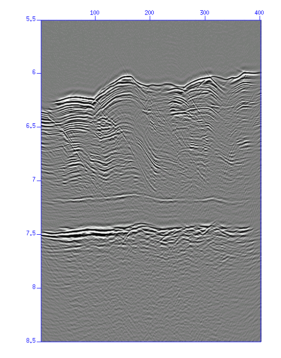
Fig: Migration results with v=1500 m/s.

Enjoy migration using some constant velocities and see how the result changes. You can change 'vmig=' manually. A shell script create_MIG_panel.sh does the job automatically. As you see at the beginning of the script,

------------------------------------
indata=Nzerooffset.su
outdata=migpanel.su
vmin=1000
vmax=2000
dv=100
------------------------------------

$ sh create_MIG_panel.sh

$ suxmovie n2=401 n3=11 loop=1 perc=98 title="Flame %g" sleep=1 < migpanel.su &

• "suxmovie" displays data in a movie.
• 'loop=2' loops forward and backward. 'loop=1' loops only forward direction. 'loop=0' never loops.
• 'sleep=' gives the time between frames in seconds.

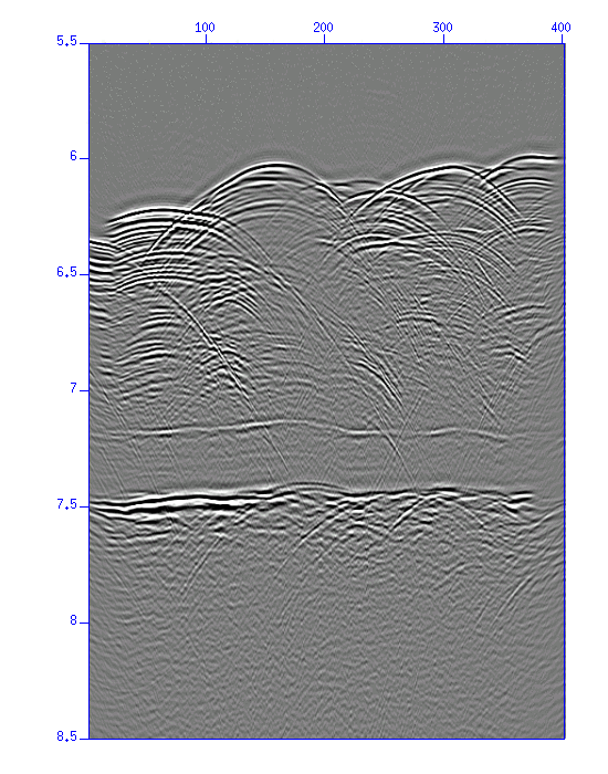
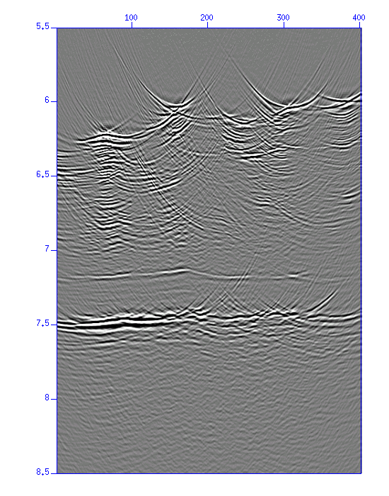
Fig: Migration results with v=1000, 1500, 2000 m/s.

To achieve a successful migration, you should create your 1-D velocity structure by referring the following information;

• Migration result with constant velocities,
• Result of "create_MIG_panel.sh",
• Velocity in "Nvpick.txt" you picked for NMO correction and the velocity structure,

$ sustolt cdpmin=900 cdpmax=1300 dxcdp=16.667 tmig=0,6,7,8,9 vmig=1500,1500,1600,1700,1800 lstaper=20 lbtaper=100 < Nzerooffset.su > Nmig.su
$ suximage < Nmig,su perc=98 &

• Stolt migtration (1978) can deal with an 1-D velocity structure.
• Velocity structure is provided using arrays like 'tmig=0,6,7,8,9 vmig=1500,1500,1600,1700,1800'. This is an example.

The migration result is the time section of the structure.

$ suttoz t=0,6,7,8,9 v=1500,1500,1600,1700,1800 < Nmig.su | suximage perc=98 &

• "suttoz" converts t (time) to z (depth).
• The 1-D velocity structure is specified as 't=0,6,7,8,9 v=1500,1500,1600,1700,1800'