Geophysical Exploration of Crustal Structure

Exercise 5

Migration

First, display the data "demo_mig1.su".

$ suximage < demo_mig1.su &

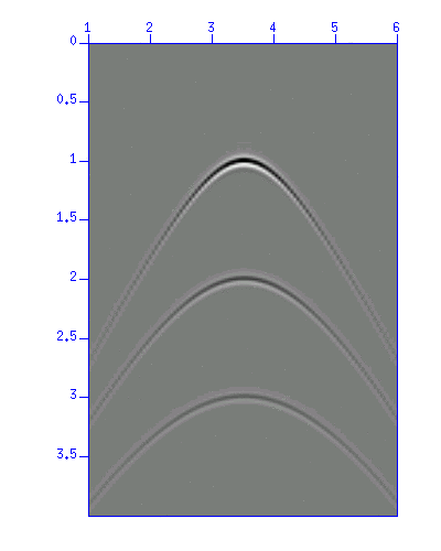
Fig: Image display of "demo_mig1.su". The vertical axis is 'time (s)' and the horizontal axis is the CMP number.

This record represents a zero-offset record with three scatterers at different depths.

Check the contents (the range of the header) of the data.

$ surange < demo_mig1.su

101 traces:
tracl    1 101 (1 - 101)
tracr    1 101 (1 - 101)
cdp      1 101 (1 - 101)    % CDP from 1 to 101
cdpt     1
trid     1
sx       0 5000 (0 - 5000)
gx       0 5000 (0 - 5000)
counit   1
ns       201
dt       19999              % dt = 2 (ms), seems strange.
d2       0.050000           % CDP interval = 0.05 (km) = 50 (m)

$ sustolt cdpmin=1 cdpmax=101 tmig=2 vmig=???? dxcdp=50 < demo_mig1.su | suximage &

• "sustolt" does time-migration by Stolt (1978).
• From header, CDP No. is from 1 to 101. Therefore set 'cdpmin=1 cdpmax=101'.
• 'd2= ' of the data is d2 = 0.050 (km) = 50 (m). Therefore, the CDP interval is 'dxcdp=50'. Mind the unit.
• 'vmig=????' carries the velocity (m/s). First, we use a constant velocity model.
• 'tmig= ' and 'vmig= ' are the pairs used to provide a velocity structure. In this case, since the velocity is constant, any value can be used, for example, 'tmig= 2' (s).

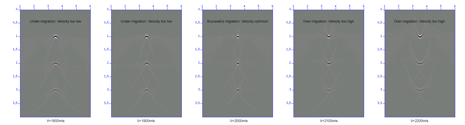
Fig: Migration results obtained using vmig=1800, 1900, 2000, 2100, 2200 (m/s).

From the results, you will see that;

• when the velocity is too small, the diffraction curves are convex upward (under-migrated).
• the curves converge when the correct velocity (2000 m/s in this case) is used,
• the diffraction curves are convex downward (over-migrated) when the velocity is too large.

Next, apply the migration to "demo_mig2.su" as well. You need to find the correct velocity value. (Hint: The velocity is constant.) You can do it manually in a try-and error approach. However, it is a clever idea to use the shell script in Exercise 4 after some modifications.

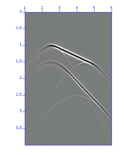
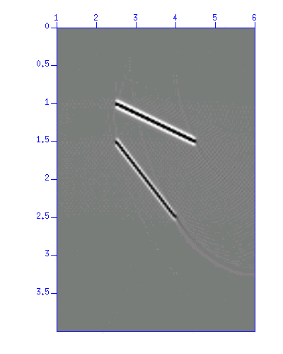
Fig: (Left) Image display of "demo_mig2.su", (Right) migrated result.

You will see that

• the diffractions from the edge of the reflectors are converged.
• the dip of the dipping reflectors is changed (more steeper).
• the location of the dipping reflectors is laterally shifted.

Next, apply the migration to "demo_mig3.su" as well.

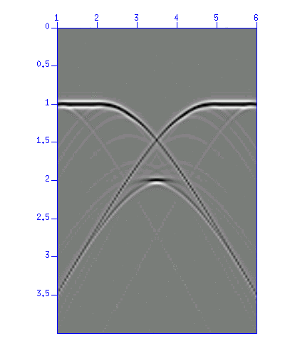
Fig: Image display of "demo_mig3.su".

The velocity is not provided here (it is also constant). Find the appropriate migration velocity, and apply the migration.

Next, apply migration to "demo_mig4.su".

Display "demo_mig4.su".

$ suximage < demo_mig4.su &

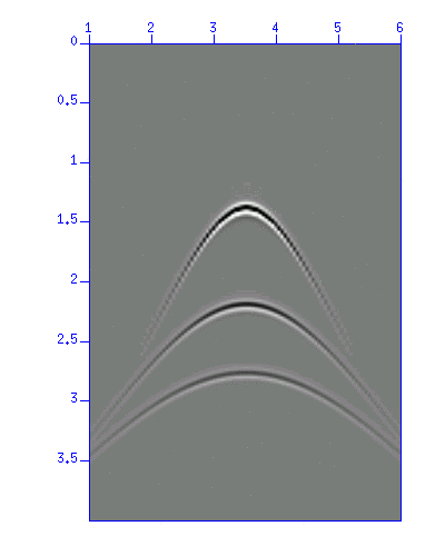
Fig: Image display of "demo_mig4.su".

The image (waveforms) of "demo_mig4.su" looks resemble that of "demo_mig1.su". This record indicates three scatterers at different depths as well as the above example. Apply migration to this record.

$ sustolt cdpmin=1 cdpmax=101 tmig=2 vmig=???? dxcdp=50 < demo_mig4.su | suximage &

Now exercising .....

You may have noticed that the three diffractions converge under the different velocity models. This is because the subsurface velocity is no more a constant.

Stolt migration works under 1-D velocity structure, i.e. depth-dependent velocity structure.

$ sustolt cdpmin=1 cdpmax=101 vmig=1400,1500,1600,1700,..... tmig=1.0,1.5,2.0,2.5,..... \
  dxcdp=50 < demo_mig4.su | suximage &

• Stolt(1978) migration works under a 1-D velocity structure.
• The velocity structure is specified as arrays of parameters, 'vmig=1400,1500,1600,1700,..... tmig=1.0,1.5,2.0,2.5,.....'.
• This pair means the velocity is 'vmig (m/s)' at the time 'tmig (s)'.
• You are clever enough not to type the above command line as it is. It gives you an error. '.....' is inappropriate ^^);.

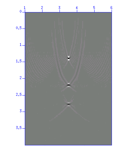
Fig: An example of the migrated "demo_mig4.su". You will reach this quality of result after some trial-and-errors.

Homework

• an image of the migrated "demo_mig3.su" and the velocity value you used to obtain the result,
• an image of the migrated "demo_mig4.su" and the 1-D velocity structure you used to obtain the result.