First, display the data (a CMP gather).
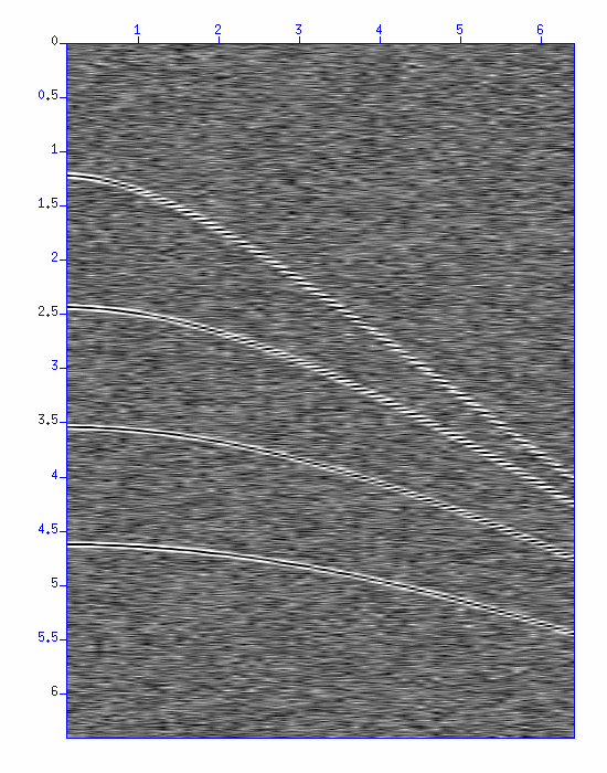
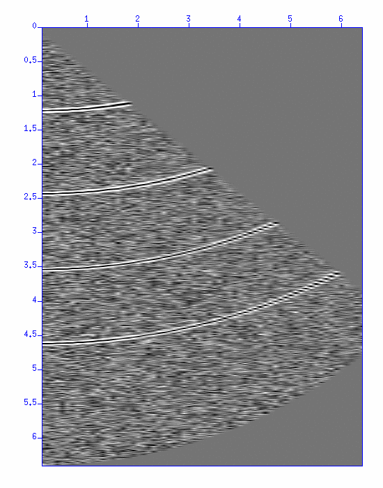
$ suximage < demo_nmo.su perc=98 &Apply normal move-out (NMO) correction with a constant velocity v=1500 m/s to this CMP gather, and display the result.
$ sunmo < demo_nmo.su vnmo=1500 | suximage perc=98 &
Fig: NMO correction, (Left) the original CMP gather, (Right) After NMO correction with a constant velocity of 1500 m/s.
Investigate how the result of NMO correction changes according to the velocity by vnmo = 1600, 1700, 1800, 1900, 2000, 2100, 2200.
$ sunmo < demo_nmo.su vnmo=1600 | suximage perc=98 &
$ sunmo < demo_nmo.su vnmo=1700 | suximage perc=98 &
......
Try a shell program create_CVS_panel.sh.html that performs Constant-Velocity-Scan (CVS). At the beginning of the script, you see,
------------------------------------
# Parameters
vmin=1200
vmax=2500
dv=50
------------------------------------
This script displays a series of NMO corrections using the velocity from 1200 m/s to 2500m/s with 50 m/s increments.
$ sh create_CVS_panel.sh
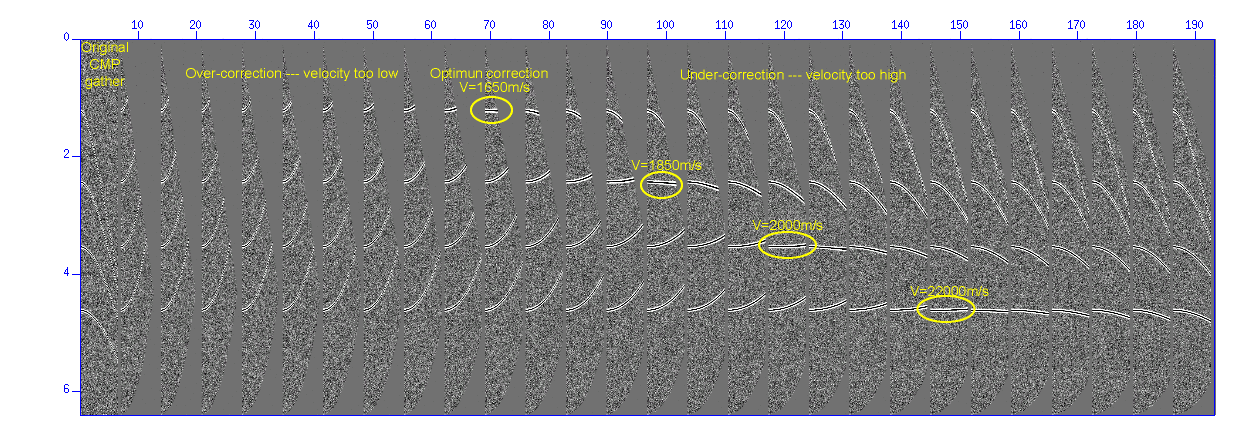
Fig: Image display of CVS panel. (Left) Original CMP gather, (Right) Result of NMO correction using the velocity from 1200 m/s to 2500m/s with the increment of 50 m/s.
NMO correction works well around the velocity = 1650, 1850, 2000, 2250 m/s. (It may not be easy to understand since the horizontal axis does not denote the velocity itself.) The stacking velocities are thus determined.
Try displaying the result in a movie.
$ suxmovie < cvspanel_demo.su n1=1601 n2=69 n3=26 loop=1 sleep=1 perc=98 &
After NMO correction, stack (sum) traces in the CDP gather. Take a look at the effect of stacking.
$ susort d2 < cvspanel_demo.su | sustack key=d2 | suxwigb &
$ susort d2 < cvspanel_demo.su | sustack key=d2 | suxwigb key=d2 &
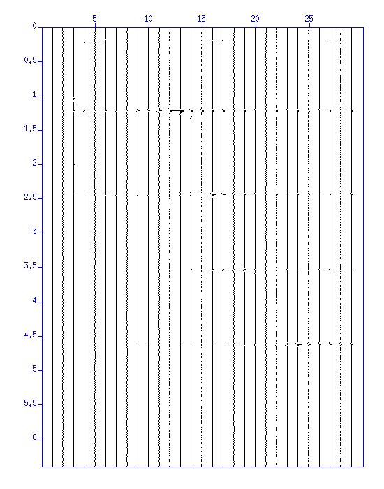
Fig: Waveform obtained by stacking after NMO correction. The horizontal axis corresponds to the velocity used for NMO correction.
Delete the file "cvspanel_demo.su" since the file is no more used.
Display a semblance panel of Constant-Velocity-Stack (CVS).
$ suvelan fv=1200 dv=50 nv=30 < demo_nmo.su | suximage f2=1200 d2=50 &
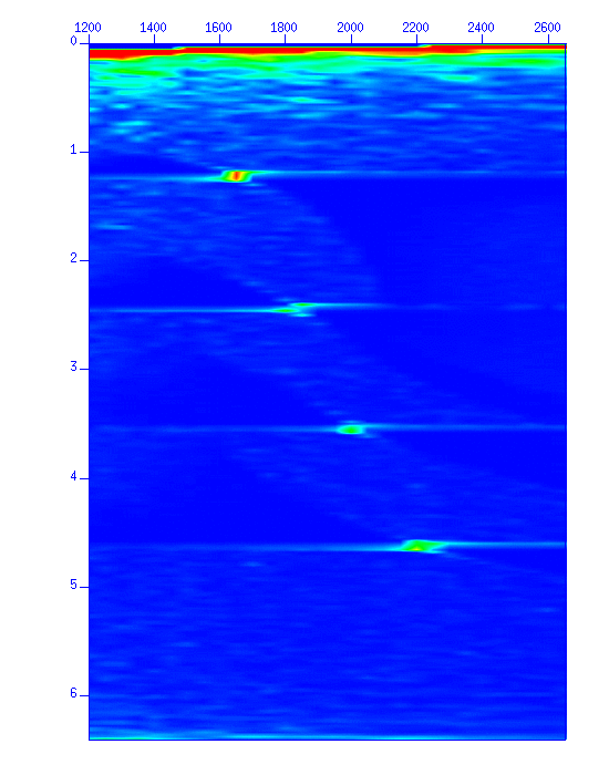
Fig: Constant-Velocity-Scan (CVS) semblance panel. The vertical axis denotes 'time (s)' and the horizontal axis denotes 'velocity (m/s)' used for NMO stacking.
By designating a file name using the option 'mpicks=filename', the mouse coordinates are written in the file when the 's' key is pressed.
$ suvelan fv=1200 dv=50 nv=30 < demo_nmo.su | suximage f2=1200 d2=50 perc=98 mpicks=pick.txt &
$ sort -n pick.txt > pick_sorted.txt
Then, change the format of the pick-file so that the picked values can be used as the input of the next step, NMO correction.
$ mkparfile < pick.txt > pick.par string1=tnmo string2=vnmoTake a look at the contents of "pick.txt" and "pick.par".
$ cat pick.txt
$ cat pick.par
$ sunmo tnmo=1.0,1.5,2.0,2.5,..... vnmo=1400,1500,1600,1700,..... < demo_nmo.su | .....We have already created a file "pick.par" containing 'tnmo' and 'vnmo'. Here we use the parameters as below.
$ sunmo par=pick.par smute=5 < demo_nmo.su | suximage perc=98 &
$ sunmo par=pick.par smute=1.5 < demo_nmo.su | suximage perc=98 &
NMO correction cause a distortion (stretch) of waveforms where the offset distance is large (in case of 'smute=5'). 'smute=' option can remove such area. In the second case, waveforms stretched 1.5 times than the original were muted ('smute=1.5').
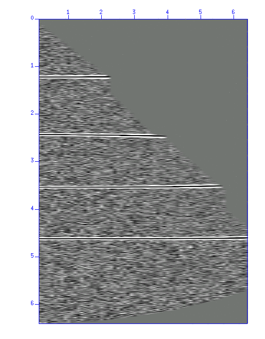
Fig: Result of NMO correction. You will see the reflected waves aligned horizontally.
Apply CDP stacking to improve S/N ratio.
$ sunmo par=pick.par < demo_nmo.su | sustack > trace.su
$ suxwigb perc=98 < trace.su &
$ suximage perc=98 < trace.su &
Stacking of the NMO corrected traces yields a single trace. Compare how the S/N ratio is improved from the original figure.
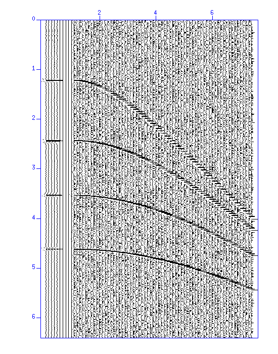
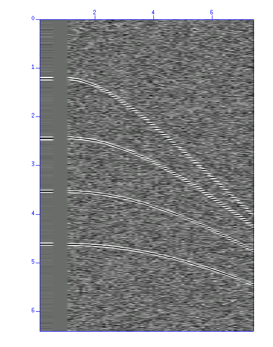
Fig: Result of NMO stacking. (Left) wiggle and (Right) image display of the waveform. In each figure, the result of stacking (5 traces) is shown on the left, and on the right is the original data. The figures show that the S/N ratio was improved.
A trace after CMP stacking is a trace that both the shot and the receiver are located at the CMP. The offset is zero. Therefore, this is called a "zero-offset trace (record)".
$ suaddnoise sn=5 < demo_nmo.su > demo_nmo_more_noise.su
Apply a velocity analysis to the data you created. Then apply NMO correction using the picked velocity values and apply CMP stack.
Submit
Tips: How to display the stacked trace and the original trace in the same amplitude scale.
If you want to align the stacked trace (5 traces) and the original traces, concatenate the data using "cat" command.
$ cat trace.su trace.su trace.su trace.su trace.su demo_nmo_more_noise.su > stacked_result_and_original.suFive stacked traces (trace.su) and the original CMP gather (demo_nmo_more_noise.su) will be displayed in one figure.
FYI
In the figures in this exercise web page, 5 null traces (zero traces) are inserted between the stacked traces and the original gather.
$ sunull ntr=5 nt=1601 > null.su
$ cat trace.su trace.su trace.su trace.su trace.su null.su demo_nmo_more_noise.su > stacked_result_and_original.su