Geophysical Exploration of Crustal Structure

Exercise 3

Vibroseis, auto-correlation and cross-correlation

In reflection seismology, a linear model;

seismic wave = source wavelet * reflection coefficient + noise

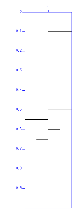
Display the reflection coefficient "demo_imp.su".

$ suxwigb < demo_imp.su &

• There are 5 impulses of reflection coefficients. In case you see no or fewer impulses, grab the window with a mouse pointer and change the size of the window.

Fig: Reflection coefficients. The vertical axis is 'time (s)'.

Then, create a sweep waveform (wave with increasing or decreasing frequency in time) which is often used by Vibroseis source, and display it.

$ suvibro f1=10 f2=100 tv=1 t1=0.1 t2=0.1 dt=0.001 > tmp_vib.su
$ suxwigb < tmp_vib.su &

• "suvibro" generates a sweep waveform of the frequency from 'f1' (Hz) to 'f2' in 'tv' seconds.
• 'dt' is the sampling time. 't1' and 't2' denote the width of the taper at the beginning and the end of the waveform.

Display the autocorrelation of the sweep waveform.

$ suacor < tmp_vib.su ntout=201 | suxwigb va=4 &
$ suacor < tmp_vib.su ntout=201 sym=0 | suxwigb va=4 &

• "suacor" calculates the autocorrelation function (ACF) of a given waveform.
• Note that the ACF is symmetrical against time. The midpoint of the time axis denotes lag time = 0.
• "sushw" set a value in a header keyword. Here we set the header keyword 'delrt' to -0.1 (s) = -100 (ms) to shift the ACF trace so that the center of the time axis meets 0.
• The option 'sym=0' generates the ACF in positive lag time only.
• This wavelet is often called a "Clauder wavelet".

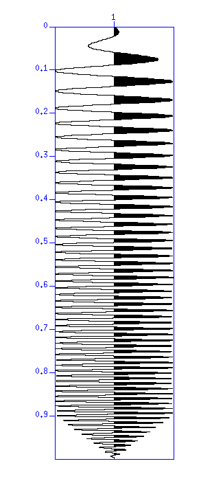
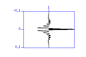
Fig: (Left) Sweep waveform from 10 to 100 Hz. The vertical axis denotes 'time (s)'. (Right) Its auto-correlation. The vertical axis is 'lag time (s)'.

Convolve the reflection coefficient with the sweep waveform, and then add noises. This simulates a seismic wave we usually observe.

$ suconv sufile=tmp_vib.su < demo_imp.su > tmp_cnv.su
$ suxwigb < tmp_cnv.su &
$ suaddnoise sn=10 < tmp_cnv.su > tmp_cnv_noise.su
$ suxwigb < tmp_cnv_noise.su &

$ suconv sufile=tmp_vib.su < demo_imp.su | suaddnoise sn=10 > tmp_cnv.su
$ suxwigb < tmp_cnv.su &

• "suconv" does convolution of the two time series.
• "suaddnoise" adds noise to data.
• 'sn=10' denotes the S/N ratio. The larger the S/N ratio is, the smaller the noises are. Try other values of 'sn= '.

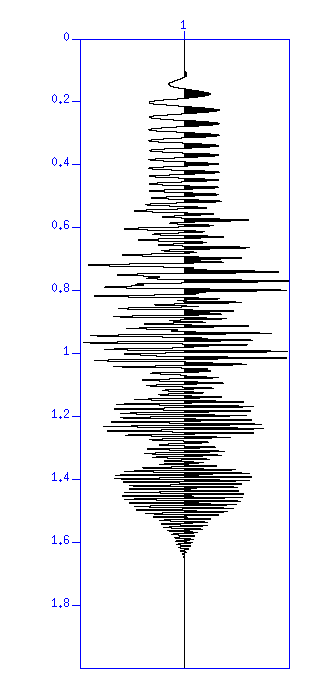
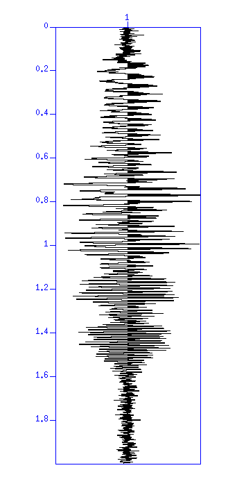
Fig: (Left) Result of convolution without noise. The vertical axis is 'time (s)'. (Right) Waveform after adding noise.

Using Vibroseis source, we observe seismic records like this.

seismic wave = source wavelet * reflection coefficient + noise

Calculate cross-correlation of the seismic record and the original sweep wavelet.

$ suxcor sufile=tmp_vib.su < tmp_cnv.su | suxwigb &

• "suxcor" does cross-correlation function (CCF or XCF) of two time series.
• The wave designated by the option 'sufile=' and the seismic data from STDIN are cross-correlated.

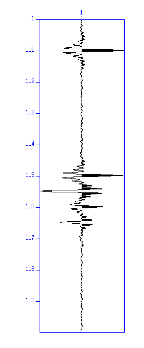
Fig: (Left) Result of cross-correlation. The vertical axis is 'time (s)'. (Right) Original reflection coefficients.

Please recall that the seismic wave is expressed as;

seismic wave = source wavelet * reflection coefficient + noise

seismic wave (xcor) source wavelet
  = (source wavelet * reflection coefficient + noise) (xcor) source wavelet
  = (source wavelet * reflection coefficient) (xcor) source wavelet + noise (xcor) source wavelet
  => auto-correlation of source wavelet (Clauder Wavelet) * reflection coefficient

Deconvolution (Predictive deconvolution)

First, display the waveform and the autocerrelation of the sample data "demo_dcn.su".

$ suxwigb < demo_dcn.su &
$ suacor < demo_dcn.su | sushw key=delrt a=-200 | suxwigb &

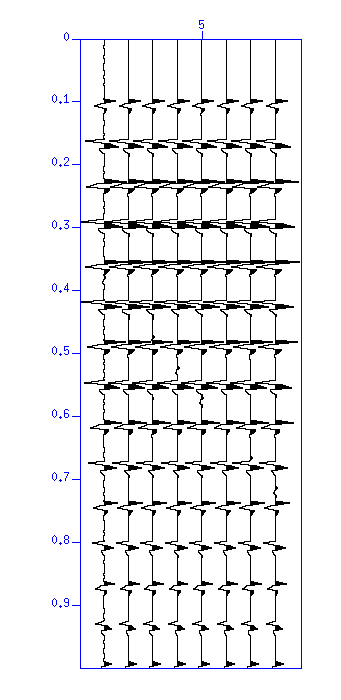
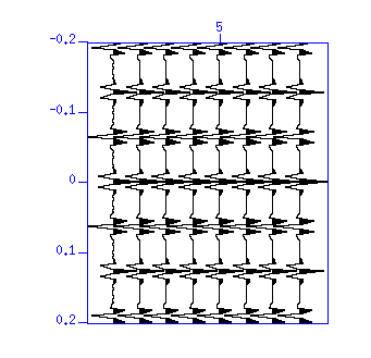
Fig: (Left) Waveform. The vertical axis is 'time (s)'. (Right) Autocorreation. The vertical axis is 'lag time (s)'.

You will see that the repetition with large amplitude is dominant in both the waveforms and the ACFs. You may also notice their polarity is alternating. This is a typical example of water reverberations often seen in the seismic record observed at shallow offshore. They usually mask weak reflections, therefore, it is important to remove these reverberations.

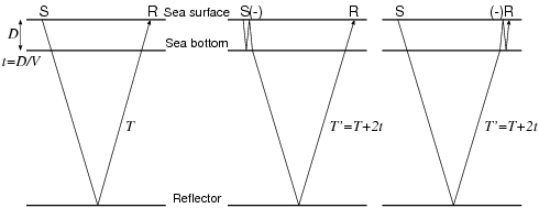
Fig: Illustration of water reverberations.

First, apply a deconvolution filter that converts the wavelet to a pulse (spike), then display the result and its auto-correlation.

$ supef < demo_dcn.su maxlag=???? > tmp_decon.su
$ suxwigb < tmp_decon.su &
$ suacor < tmp_decon.su | sushw key=delrt a=-200 | suxwigb &

• "supef" applies a Predictive Error Filter (PEF). (Whitening/spiking) deconvolution is a special case of the PEF.
• 'maxlag' denotes an operator length (s) of the filter. It is not always easy to find an appropriate value for 'maxlag'. Auto-correlation gives information.

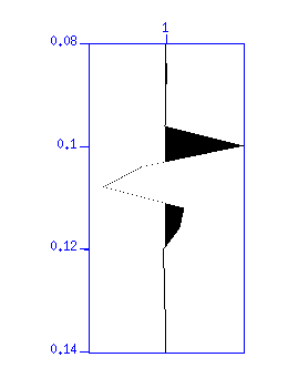
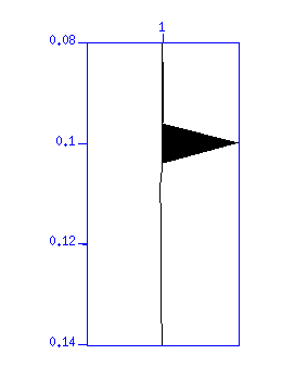
Fig: (Left) Original wavelet (enlargement), (Right) Result of deconvolution.

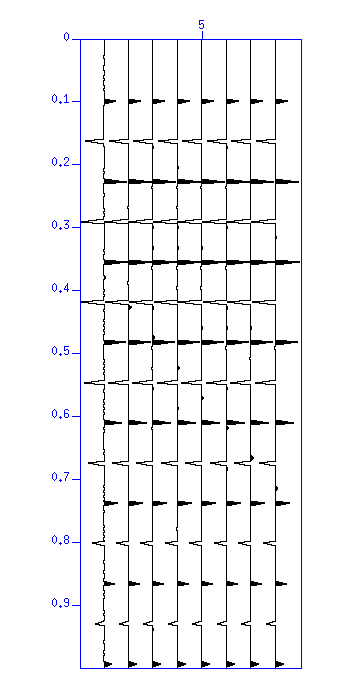
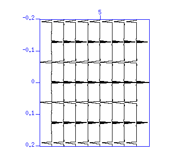
Fig: (Left) Result of deconvolution. The vertical axis is 'time (s)'. (Right) Autocorreation. The vertical axis is 'lag time (s)'. Pulsive autocorrelation shows that the wavelet was converted to a pulse.

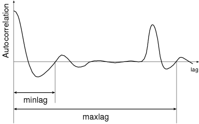
Next, apply a PEF that removes the repeated feature in the waveform.

$ supef minlag=???? maxlag=???? < tmp_decon.su | suxwigb &
$ supef minlag=???? maxlag=???? < tmp_decon.su | suacor | sushw key=delrt a=-200 | suxwigb &

Try the optimum value for 'minlag' and 'maxlag' using;

• From 0.01 to 0.10 (s) for 'minlag= '
• From 0.10 to 0.20 (s) for 'maxlag= '

If your values are appropriate, the repetition will be removed. A signal indicating dipping layers, which is masked by the water reverberations, will appear as shown in the figures below.

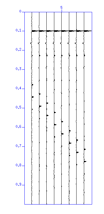
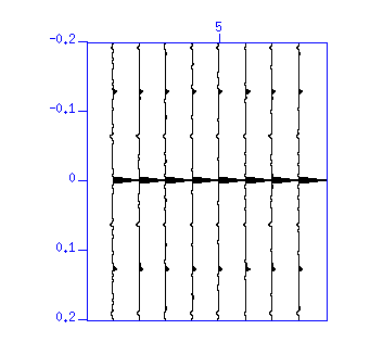
Fig: (Left) Result of deconvolution. The vertical axis is 'time (s)'. (Right) Autocorrelation. The vertical axis is 'lag time (s)'. Autocorrelation also shows that the repetitions are removed.

In usual data processing, a band-pass filter is applied after deconvolution to recover the original spectrum band from the whitened (broadened) spectrum by deconvolution.

Homework

• the optimum value for "maxlag" in order to do spiking the wavelet,
• the optimum value for "minlag" and "maxlag" in order to remove reverberations,
• figures of the waveform after applying deconvolutions,
• and its auto-correlation.