First, display the waveform of the sample data.
$ suxwigb < demo_bpf.su perc=98 &Display the spectrum of the data.
$ suspecfx < demo_bpf.su | suximage perc=98 &
$ suspecfx < demo_bpf.su | suxgraph &
$ suspecfx < demo_bpf.su | suop op=db | suxgraph &
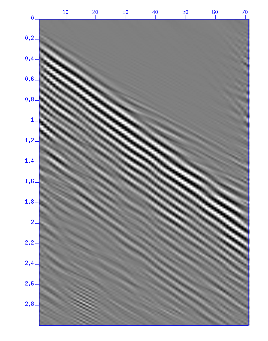
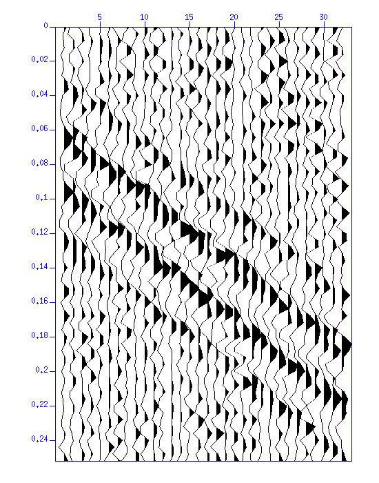
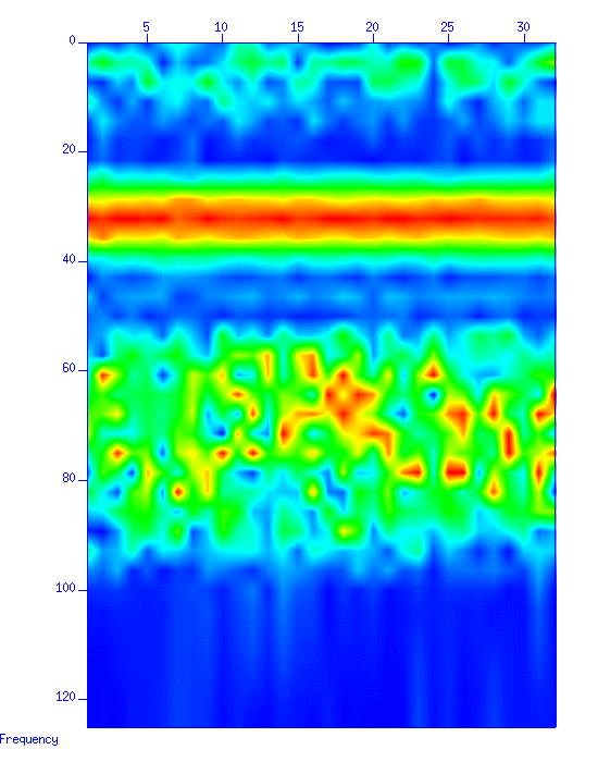
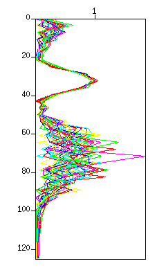
Fig: (Left) The waveform. The vertical axis is 'time (s)'. (Middle) The spectrum in a color image. The vertical axis is 'frequency (Hz)'. (Right) The spectrum in a graph style.
Then, apply some frequency filters and display the result.
From the spectrum, you can find three frequency bands, < 20 Hz, 20 - 40 Hz, 50 - 100 Hz in the data. Therefore, here we will apply filters shown in the following figure.
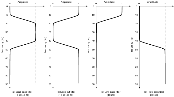
First, extract the signal of 20 - 40 Hz by applying the bandpass filter (a).
$ sufilter f=10,20,40,50 amps=0,1,1,0 < demo_bpf.su | suxwigb &
$ sufilter f=10,20,40,50 amps=0,1,1,0 < demo_bpf.su | suspecfx | suxgraph &
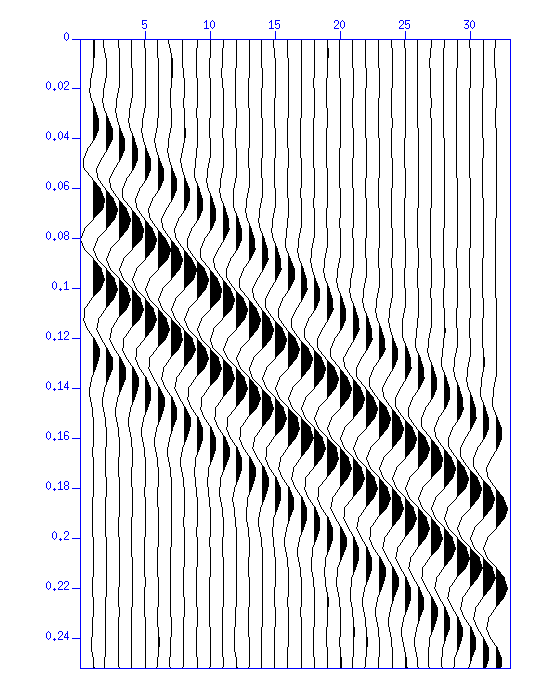
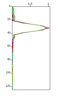
Fig: (Left) The waveform. The vertical axis is 'time (s)'. (Right) The spectrum in a graph style. The vertical axis is 'frequency (Hz)'.
Make sure that the signal of 20 - 40 Hz remains while other frequenciy bands diminish.
The filter (b) removes the frequency band of the filter (a). Note the option 'amps='.
$ sufilter f=10,20,40,50 amps=1,0,0,1 < demo_bpf.su | suxwigb &
$ sufilter f=10,20,40,50 amps=1,0,0,1 < demo_bpf.su | suspecfx | suxgraph &
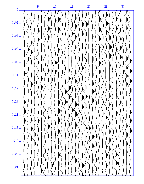
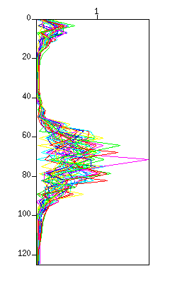
Fig: (Left) The waveform. The vertical axis is 'time (s)'. (Right) The spectrum in a graph style. The vertical axis is 'frequency (Hz)'.
Note that that the signal of 20 - 40 Hz is removed.
(c) and (d) are the low-pass and the high-pass filters, respectively.
$ sufilter f=10,20 amps=1,0 < demo_bpf.su | suxwigb &
$ sufilter f=10,20 amps=1,0 < demo_bpf.su | suspecfx | suxwigb &
$ sufilter f=40,50 amps=0,1 < demo_bpf.su | suxwigb &
$ sufilter f=40,50 amps=0,1 < demo_bpf.su | suspecfx | suxwigb &
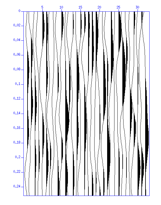
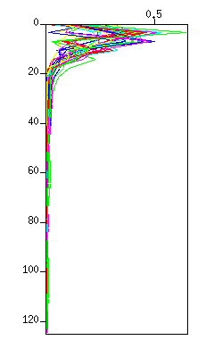
Fig: (Left) The waveform. The vertical axis is 'time (s)'. (Right) The spectrum displayed in graph style. The vertical axis is 'frequency (Hz)'.
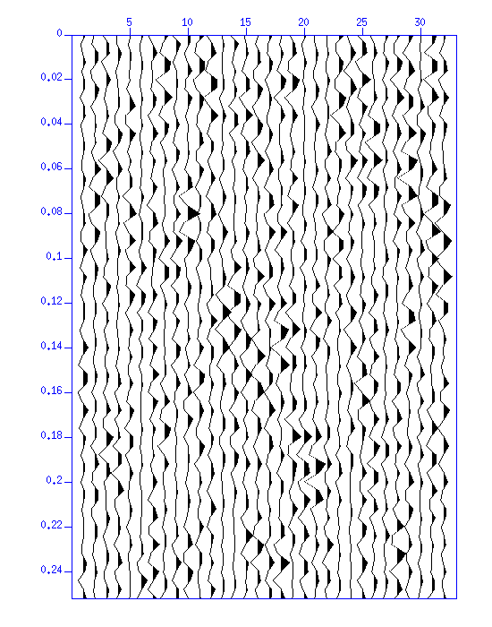
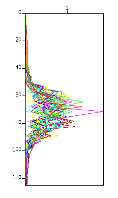
Fig: (Left) The waveform. The vertical axis is 'time (s)'. (Right) The spectrum in a graph style. The vertical axis is 'frequency (Hz)'.
Note the pass-band and the cut-band of each filter.
First, display the waveform.
$ suxwigb < demo_fkf.su &You will see three waves having different apparent velocities. Note that the wave crosses with each other.
Calculate "double Fourier transform" to convert time-space (t-x) data to frequency-wavenumber (f-k) data, and display the f-k spectrum.
$ suspecfk < demo_fkf.su | suximage &
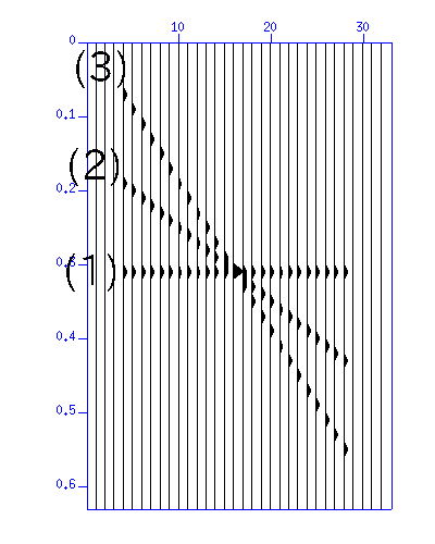
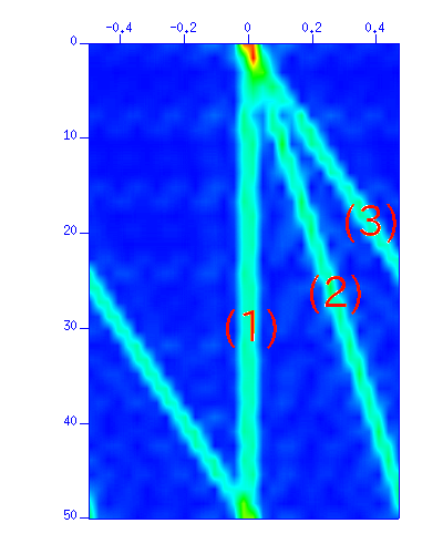
Fig: (Left) The waveform. The vertical axis is 'time (s)'. The horizontal axis is 'distance (m)'. (Right) The f-k spectrum in a color image. The vertical axis is 'frequency (Hz)'. The horizontal axis is 'wavenumber (1/m)'.
Waves (1),(2),(3) in t-x plane are converted to the images indicated by the number in f-k plane. Note that the wave (3) are spatially aliased (wrap-around in the wavenumer domain).
Now apply the velocity filters. From the waveforms in t-x plane, the dip (dt/dx) of the waves (1), (2), (3) are 0.00, 0.01, 0.02, respectively.
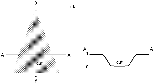
First, try eliminating the wave (1). Since the dip (dt/dx) of the wave is zero (0) in t-x plane (the apparent velocity is infinity), apply a filter that removes the energy around the zero dips (-0.005 - 0.005). In f-k plane, the filter looks like the one in the following figure.
sudipfilt slopes=-0.01,-0.005,0.005,0.01 amps=1,0,0,1 < demo_fkf.su | suxwigb  &
sudipfilt slopes=-0.01,-0.005,0.005,0.01 amps=1,0,0,1 < demo_fkf.su | suspecfk | suximage &
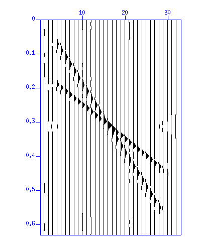
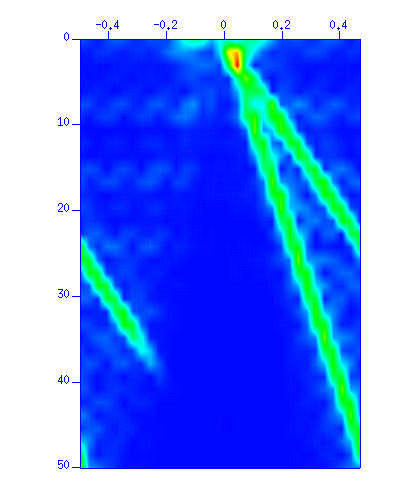
Fig: (Left) The waveform. The vertical axis is 'time (s)'. The horizontal axis is 'distance (m)'. (Right) The f-k spectrum in a color image. The vertical axis is 'frequency (Hz)'. The horizontal axis is 'wavenumber (1/m)'.
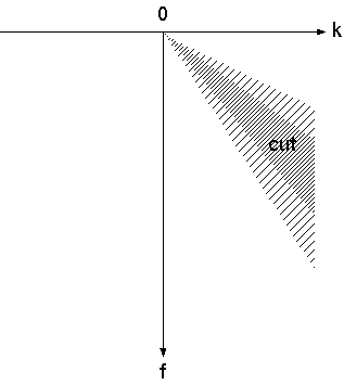
Next, try eliminating the wave (3). Since the dip (dt/dx) of the wave is 0.02 in t-x plane, apply a filter that removes the energy around dip=0.02 (0.0175 - 0.0225). In f-k plane, the filter is shown in the following figure.
sudipfilt slopes=0.015,0.0175,0.0225,0.025 amps=1,0,0,1 < demo_fkf.su | suxwigb &
sudipfilt slopes=0.015,0.0175,0.0225,0.025 amps=1,0,0,1 < demo_fkf.su | suspecfk | suximage &
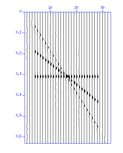
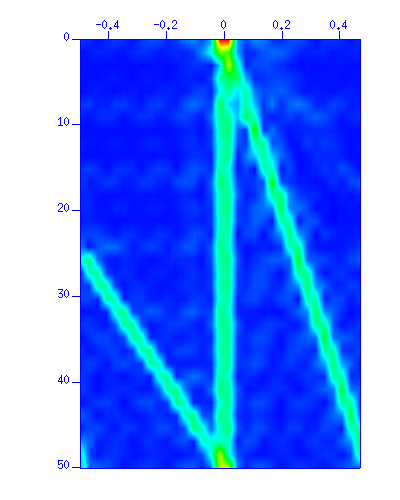
Fig: (Left) The waveform. The vertical axis is 'time (s)'. The horizontal axis is 'distance (m)'. (Right) The f-k spectrum in a color image. The vertical axis is 'frequency (Hz)'. The horizontal axis is 'wavenumber (1/m)'.
Note that the filter failed to remove the wave (3) completely in t-x plane. The reason is clear in f-k plane. The filter did not cover the alised part of the wave (3) in the negative wavenumber. To remove the wave (3) completely, you will need to apply a filter that removes the negative wavenumber as well. As spatial aliasing cause problems in data processing, you will need care in deciding the number of receivers and their separation distance.
sudipfilt slopes=(slopes to be removed from the figure of the waveforms) amps=?,?,?,? < demo_fkf2.su | .............In this example, use the time scale in the display of the waveform image to calculate the slope.
Submit
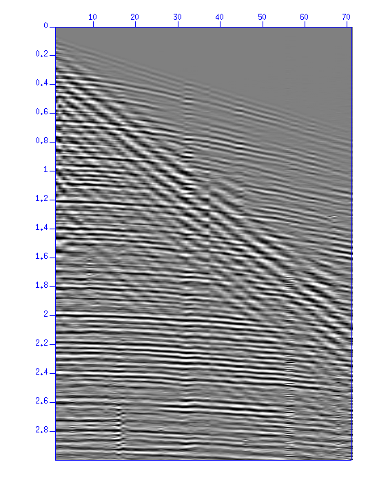
Fig: (Left) Sample data "demo_fkf2.su". The vertical axis is the time (s). The horizontal axis is the distance (m).
The result after PRESERVING the surface wave only, just for your reference.