waterPMLコマンドの検証

3. 傾いた斜面での傾斜変動の計算

(Examples and validations for waterPML command — 3. computation of tilt changes on a slope)


◆概要とコマンド (Outline and the command)

waterPMLコマンドの検証の3つ目として、 一定角度で傾いた斜面上での傾斜変動の計算について述べる。 これはMaeda et al. (2021)の3.4節に対応する。 コマンドの例を以下に示す。
As the 3rd examination of the waterPML command, consider to compute the tilt changes on a slope of a constant angle. This example corresponds to Section 3.4 of Maeda et al. (2011). An example of the command is shown below.

waterPML --Nx=101 --Nz=51 --Npmx=10 --x0=-505.0 --y0=-505.0 --z0=-400.0 --dx=10.0 --dt=0.001 --tmax=10.0 --structure_file=structure.ini --structure_file_format=layer --source_file=source3.ini --output_dir=result03 --station_file=station_list3.dat --topography_files=topography_constant_slope.dat --topography_file_format=xy

2つ目の例題と異なる部分を色で示した。 青はファイル名の違いであり、赤はその他の違いを表す。 ファイル名以外で異なるのは物理領域の\(z\)座標の範囲であり、 ここでは\(-400\leq z\leq 110\) (単位:m)としている。
Here, the colors indicate differences from the 2nd example; blue show differences in file names, and red show the other differences. Except for the file names, the command is different from that of the 2nd example only in the \(z\) range of the physical volume (\(-400\leq z\leq 110\) (unit: m) in this case).


●地形データ (A topography data)

ここでは\(x\)の値が6 m大きくなる毎に標高が1 m大きくなる勾配を与える。 この場合、地表面の勾配は9.46°となる。 対応する地形データは物理領域の\((x,y)\)座標範囲を囲む4地点で 以下のように与えれば良い。
Here, let us use an inclined ground surface that increases its elevation by 1 m for every 6 m of the increment of \(x\). The corresponding slope of the ground surface is 9.46°. This topography can be given by the data below, in which elevations at the four points that bound the \((x,y)\) range of the physical volume are given.

(topography_constant_slope.dat)
-600.0[TAB]-600.0[TAB]-100.0
-600.0[TAB]600.0[TAB]-100.0
600.0[TAB]-600.0[TAB]100.0
600.0[TAB]600.0[TAB]100.0


●地震波動ソース (Seismic wave source)

Maeda et al. (2011)の3.4節に従い、 (0,0,-195)の位置に等方ソースを置く。
Following Section 3.2 of Maeda et al. (2011), an isotropic source is placed at (0,0,-195).

(source3.ini)
newsource isotropic
location_x=0.0
location_y=0.0
location_z=-195.0
mechanism=isotropic
intensity=1.0
stfun_name=pow5
stfun_tp=5.0


●観測点リスト (Station list)

\(y=0\) mおよび\(y=200\) mの測線に沿って 地表直下の全ての格子セルに観測点を置く。
Stations are placed at every grid cell immediately beneath the ground surface along \(y=0\) and \(y=200\) m transects.

(station_list3.dat)
y0_x-500[TAB]-500.0[TAB]0.0[TAB]surface-0.1
y0_x-490[TAB]-490.0[TAB]0.0[TAB]surface-0.1
y0_x-480[TAB]-480.0[TAB]0.0[TAB]surface-0.1

y0_x500[TAB]500.0[TAB]0.0[TAB]surface-0.1
y200_x-500[TAB]-500.0[TAB]200.0[TAB]surface-0.1
y200_x-490[TAB]-490.0[TAB]200.0[TAB]surface-0.1
y200_x-480[TAB]-480.0[TAB]200.0[TAB]surface-0.1

y200_x500[TAB]500.0[TAB]200.0[TAB]surface-0.1

このファイルはbashの以下のコマンドを使って容易に作成できる。
This file can be created easily by the bash command shown below.

rm -f station_list3.dat

for((x=-500;x<=500;x+=10))
do
   /bin/echo -e "y0_x${x}\t${x}.0\t0.0\tsurface-0.1" >> station_list3.dat
done

for((x=-500;x<=500;x+=10))
do
   /bin/echo -e "y200_x${x}\t${x}.0\t200.0\tsurface-0.1" >> station_list3.dat
done

観測点の標高は地表の0.1 m下(surface-0.1)とした。 観測点位置は最寄りの格子セル中心点で近似されるので、 10 mサイズの格子セルを用いる今回の計算では 実際には地表の5 m下での傾斜変動が計算されることになる。 したがってsurface-5.0と書いても結果は同じであるが、 surface-0.1と書いておけば 格子セルのサイズを変えて計算する場合に観測点リストを作り直さずに済む。
The station elevations are given as 0.1 m below the ground surface (surface-0.1). Actually, the station locations are approximated at the center of the nearest grid cell, which is 5 m below the ground surface in this case there the grid cell size is 10 m. Therefore, writing as surface-5.0 gives the same results. An advantage of writing as surface-0.1 is that the station list can be used without modification if you change the grid cell size.


◆計算後のデータの加工 (Postprocessings to arrange the results)

●傾斜変動レートの時系列データから傾斜レートの時系列データへの変換 (Transformation from tilt-rate to tilt time series data)

上記のコマンドを実行するとresult03/waveformディレクトリの下に 観測点位置における速度や傾斜変動レートの時系列データファイルが作成される。 「観測点名.Tx.seq1」が傾斜変動レートの\(x\)成分、 「観測点名.Ty.seq1」が傾斜変動レートの\(y\)成分である。 まずはこれらを積分して傾斜変動の時系列データにする。
After the calculation of the command shown above finishes, there are time series data files for velocities and tilt-rates at station locations under a directory result03/waveform. Files named “station name.Tx.seq1’ and “station name.Ty.seq1’ are the time series data for \(x\)- and \(y\)-components of the tilt-rate, respectively. First, integrate them to obtain time series data for tilt.

cd result03/waveform
for inputfile in *.Tx.seq1 *.Ty.seq1
do
   outputfile=`echo $inputfile | sed "s/.seq1/.int.seq1/"`
   sequencefile_integral $inputfile $outputfile
done

これにより、例えば 位置\((x,y)=(200,0)\)での傾斜変動レートの\(x\)成分(ファイルy0_x200.Tx.seq1) を積分した結果(傾斜変動の時系列データ)が y0_x200.Tx.int.seq1のファイル名で出力される。
By this, the \(x\)-component of tilt-rate at a location \((x,y)=(200,0)\) (file y0_x200.Tx.seq1), for example, is integrated to have a time series data for tilt that is written into a file y0_x200.Tx.int.seq1.

●5つの格子セルでの傾斜変動の平均 (Averaging the tilt at five grid cells)

Maeda et al. (2011)では階段近似した地形の段差の影響を低減するため、 観測点を中心とする隣接する5つの格子セルでの傾斜変動を平均して用いることを推奨している。 平均の傾斜変動の計算には sequencefiles_averageコマンド が利用できる。 以下は\(y=0\)の測線に沿った傾斜変動の\(x\)成分についての平均操作の例である。
Maeda et al. (2011) recommends to average the tilt changes at five adjacent grid cells centered on each station to suppress the effects of steps in the approximated topography. The average can be computed by sequencefiles_average command. Shown below is an example of the average operation for \(x\)-component tilt changes along the transect of \(y=0\).

for((x=-480;x<=480;x+=10))
do
  ((xm2=x-20))
  ((xm1=x-10))
  ((xp1=x+10))
  ((xp2=x+20))

  file1=y0_x${xm2}.Tx.int.seq1
  file2=y0_x${xm1}.Tx.int.seq1
  file3=y0_x${x}.Tx.int.seq1
  file4=y0_x${xp1}.Tx.int.seq1
  file5=y0_x${xp2}.Tx.int.seq1

  sequencefiles_average --inputfiles=$file1,$file2,$file3,$file4,$file5 --outputfile=y0_x${x}.Tx.int.ave5.seq1
done

これにより、例えば
の平均がy0_x200.Tx.int.ave5.seq1のファイル名で出力される。
By this, the tilts at the following five locations:
for example, are averaged and the result is written in a file y0_x200.Tx.int.ave5.seq1.


◆計算結果の評価 (Evaluation of the computation results)

今回の計算では一定角度で傾いた地表面を用いたので、 茂木モデル(Mogi 1958)を座標回転して得られる解析解との比較により 計算結果を評価できる。
Because the computation used a ground surface of a constant slope, the result can be evaluated by comparison with an analytical solution of Mogi (1958)'s model after rotating the coordinate.

●最終時刻での傾斜の値の取得 (Extracting the values of tilt at the final time step)

今回の計算では傾斜変動レートが時刻\(t<10\) sでほぼ0に収束したことから \(t=10\) s(最終時刻)での傾斜変動が永久に残る(静的な傾斜変動)と判断できる。 そこで、最終時刻での傾斜の値を取り出す。
The tilt-rates converted to almost zero before 10 s in this computation, suggesting that the tilt at \(t=10\) s (the final time step) will remain permanently (i.e., a static tilt). Therefore, extract the values of tilt at the final time step.

rm -f permanent_tilt.dat
for((x=-480;x<=480;x+=10))
do
  tilt1=`tail -n 1 y0_x${x}.Tx.int.seq1`
  tilt5=`tail -n 1 y0_x${x}.Tx.int.ave5.seq1`
  /bin/echo -e "$x\t$tilt1\t$tilt5" >> permanent_tilt.dat
done
cd ../..


●解析解の計算 (Computation of analytical solution)

一定角度で傾いた地表面は座標回転によって水平な地表面に変換できるので、 茂木モデルに基づいて解析解を計算できる。 ymaeda_opentoolsにおいて茂木モデルの解析解は Mogiコマンド を用いて計算できる。 以下がコマンドの例である。 Mogiコマンドにおけるパラメータsource_amplitudeの値は \(M_0/(4\pi\mu)\)であり、 waterPMLコマンドの計算に合わせて 地震モーメント\(M_0=1\) N m, 剛性率\(\mu=\rho V_s^2=\rho V_p^2/3\), 密度\(\rho=2500\) kg/m\(^3\), P波速度\(V_p=2000\) m/s とした。
Because a ground surface of a constant slope can be arranged to a flat ground surface by rotation of coordinates, an analytical solution of this problem is available from the Mogi model. A Mogi command of ymaeda_opentools computes the analytical solution. An example of the command is shown below.
The value of parameter source_amplitude of Mogi command is given as \(M_0/(4\pi\mu)\), where a seismic moment \(M_0=1\) N m, a rigidity \(\mu=\rho V_s^2=\rho V_p^2/3\), a density \(\rho=2500\) kg/m\(^3\), and a P-wave velocity \(V_p=2000\) m/s were used to be consistent with the computation by the waterPML command.

source_amplitude=`echo 2500.0 2000.0 | awk '{ mu=$1*$2*$2/3.0; printf("%e",1.0/(4.0*3.1415926*mu)) }'`

Mogi --source_location=0.0,0.0,-195.0 --source_amplitude=$source_amplitude --station_list_file=station_list3.dat --z0=0.0 --slope_x=9.46 --outputfile=result03_check/analytical_solution.dat


●比較図のプロット (Comparison of the numerical and analytical solutions)

以上で数値解(result03/waveform/permanent_tilt.dat)と 解析解(result03_check/analytical_solution.dat)の 傾斜変動の空間分布の数値データが得られた。 これらをグラフとしてプロットすることは容易であり、例えば Generic Mapping Tools (version 6) を用いて以下の手順でプロットできる。
Numerical (result03/waveform/permanent_tilt.dat) and analytical (result03_check/analytical_solution.dat) solutions for the spatial distribution of tilt have been obtained as numerical data. They can easily be plotted, for example by Generic Mapping Tools (version 6) as below.

mkdir result03_tilt_comparison

cd result03_tilt_comparison

gmt begin comparison ps

gmt set FONT_ANNOT_PRIMARY 12p

grep y0_ ../result03_check/analytical_solution.dat | awk '{ print $7,$5*1e+18 }' | gmt plot -R-500/500/-4.5/4.5 -JX10/7 -Xa3 -Ya3 -W2,150/150/150

awk '{ print $1,$2*1e+18 }' ../result03/waveform/permanent_tilt.dat | gmt plot -R-500/500/-4.5/4.5 -JX10/7 -Xa3 -Ya3 -W1,0/0/255

awk '{ print $1,$3*1e+18 }' ../result03/waveform/permanent_tilt.dat | gmt plot -R-500/500/-4.5/4.5 -JX10/7 -Xa3 -Ya3 -W1,255/0/0 -Bxa200f100 -Bya2f1 -BWSen

gmt text -R0/21/0/29.7 -JX21/29.7 -Xa0 -Ya0 -F+f12p+a+j <<EOF
8.0 2.3 0 CT x (m)
2.2 6.5 90 CB Tilt (10@+-18@+ rad)
EOF

gmt end

ここでは\(y=0\)の断面における傾斜変動の\(x\)成分をプロットしている。 上記のコマンドを実行すると図1のグラフが生成される。 Maeda et al. (2011)の図7cに対応するものである。 但し1つ目の例と同様、 用いたS波速度の値がMaeda et al. (2011)とは僅かに異なるので 厳密に同じものではない。 waterPMLコマンドの計算結果(青)には 地形を階段状に近似した影響が現れているが、 隣接する5つの格子セルでの傾斜変動の平均(赤)を求めることで 地形の近似の影響が低減されていることが分かる。
This example plots the \(x\)-component of tilt along a transect of \(y=0\). The result is Fig. 1 and corresponds to Fig. 7c of Maeda et al. (2011); however, the data in the two figures are not exactly identical because of a slight difference in S-wave velocities used, as described in the 1st example. The computation result from the waterPML command (blue) shows an effect of stepwise approximation of topography; this effect is reduced in the 5 grid cell averages of tilt (red).


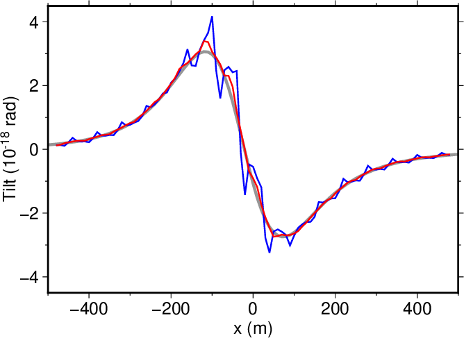
図1. \(y=0\)の断面における傾斜変動の\(x\)成分。 灰色は茂木モデルに基づく解析解、 青はwaterPMLコマンドによる数値解である。 数値解を隣接する5つの格子セルで平均した結果を赤で示す。
Fig. 1. The \(x\)-component of tilt along a transect of \(y=0\). Gray and blue lines show an analytical solution from the Mogi model and a numerical solution from the waterPML command, respectively. The red line show the numerical solution averaged over adjacent five grid cells.