waterPMLコマンドの検証

2. 半無限媒質での計算

(Examples and validations for waterPML command — 2. computation in a half space)


◆概要とコマンド (Outline and the command)

waterPMLコマンドの2つ目の使用例として、 水平な地表面を持つ半無限媒質での計算について述べる。 これはMaeda et al. (2011)の3.2節に対応する。 コマンドの例を以下に示す。
As the 2nd example of the use of the waterPML command, consider to compute the wave field in a half space medium under a flat ground surface. This example corresponds to Section 3.2 of Maeda et al. (2011). An example of the command is shown below.

waterPML --Nx=101 --Npmx=10 --x0=-505.0 --y0=-505.0 --z0=-1000.0 --dx=10.0 --dt=0.001 --tmax=10.0 --structure_file=structure.ini --structure_file_format=layer --source_file=source2.ini --output_dir=result02 --station_file=station_list2.dat --topography_files=topography_flat.dat --topography_file_format=xy

1つ目の例と異なる部分を色で示した。 青はファイル名の違いであり、赤はその他の違いを表す。
Here, the colors indicate differences from the 1st example; blue show differences in file names, and red show the other differences.


●地形データ (A topography data)

1つ目の例(無限媒質)との一番の違いは地形データを用いる点であり、 --topography_files=topography_flat.dat --topography_file_format=xy のオプションでこの指定を行っている。 今回の例では水平な地表面であるので 物理領域を囲む4地点で地表面の標高を定義すれば良い。 したがって例えば次のようなファイルを用意する。
The most essential difference between this and former (infinite medium) examples is the use of a topography data specified by --topography_files=topography_flat.dat and --topography_file_format=xy options. The topography data must be defined at four points that bound the physical volume to express a flat ground surface. Therefore, prepare a file shown below.

(topography_flat.dat)
-600.0[TAB]-600.0[TAB]0.0
-600.0[TAB]600.0[TAB]0.0
600.0[TAB]-600.0[TAB]0.0
600.0[TAB]600.0[TAB]0.0

これにより、4地点(-600,-600), (-600,600), (600,-600), (600,600)において いずれも地表面の標高が0であるという指定になる。 プログラム内でこのデータの補間が自動的に行われ、 物理領域内の全ての地点において地表面が標高0 mに設定される。
This file indicates that the ground surface is at 0 m elevation at four points (-600,-600), (-600,600), (600,-600), and (600,600). This data is automatically interpolated in the program, and the result is a ground surface of 0 m elevation throughout the entire physical volume.


●格子セルサイズと時間刻み (Grid cell size and time stepping)

計算精度を上げるために格子サイズを10 mとし、 \((x,y)=(0,0)\)が格子セル中心点になるように 物理領域の範囲を\(-505\leq x,y\leq 505\) (単位:m)とした。 また、\(z=0\) mに地表面を置く都合上、 \(z=0\)が格子セルの境界になるように \(-1000 \leq z\leq 10\)とした。 \(z\)の最大値が0ではなく10なのは 最低でも1つの真空セルが無いと地表面を表現できないからである。
To improve the computation accuracy, a grid cell size of 10 m is used. Corresponding to this change, the \(x\) and \(y\) ranges of the physical volume were changed to \(-505\leq x,y\leq 505\) (unit: m) to keep the origin (\((x,y)=(0,0)\)) at the center of a grid cell. In contrast, \(z=0\) must be at the boundary of grid cells because the ground surface must be placed there. For this reason, the \(z\) range of the physical volume was given as \(-1000 \leq z\leq 10\). The upper limit of \(z\) is not 0 but 10 because at least one grid cell in the vacuum is needed to express the ground surface.

経験上、計算の時間刻み(s)は格子セルサイズ(m)の1/10000以下にしないと数値不安定が発生する。 そのため格子セルサイズを10 mに変更したのに合わせて時間刻みを0.001 sとした。
My experiences indicate that the time stepping (s) must be less than or equal to 1/10000 times the grid cell size (m) to avoid numerical instability. For this reason, a time stepping of 0.001 s was used corresponding to the grid cell size of 10 m.


●地震波動ソース (Seismic wave source)

Maeda et al. (2011)の3.2節に従い、 (0,0,-505)の位置に等方ソースを置く。 そのために設定ファイルは以下のように記載する。
Following Section 3.2 of Maeda et al. (2011), an isotropic source is placed at (0,0,-505). This setting is realized by writing the configuration file as follows.

(source2.ini)
newsource isotropic
location_x=0.0
location_y=0.0
location_z=-505.0
mechanism=isotropic
intensity=1.0
stfun_name=pow5
stfun_tp=5.0


●観測点リスト (Station list)

観測点は\((x,y)=(200,0)\)とし、 地表からの深さ5 m, 15 m, 25 m, 35 mに置く。 したがって観測点リストファイルは以下のようになる。
The stations are located at \((x,y)=(200,0)\), with depths of 5, 15, 25, and 35 m from the ground surface. Therefore, the station list file is as below.

(station_list2.dat)
d5[TAB]200.0[TAB]0.0[TAB]surface-5.0
d15[TAB]200.0[TAB]0.0[TAB]surface-15.0
d25[TAB]200.0[TAB]0.0[TAB]surface-25.0
d35[TAB]200.0[TAB]0.0[TAB]surface-35.0

この例の第4列が示すように、 地表面のある計算では観測点の標高を「地表の下何m」という形式で指定できる。 このようにすれば実際の3次元データを用いた計算の際に 地表面の標高を調べずに済むので便利である。
As the 4th column of this example shows, the station elevations can be specified in the form of depth from the ground surface. This option is comvenient, as the users do not need to survey the station altitudes in case of using real 3-D topography.


◆計算結果の評価 (Evaluation of the computation results)

●波数積分法の計算結果のファイル (Files for computation results by a discrete wavenumber method)

Maeda et al. (2011)の3.2節にならい、 ここでもwaterPMLコマンドによる計算結果を武尾(1985)の波数積分法による結果と比較する。 波数積分法のプログラムは著者のコードではなく公開できないため計算結果のファイルを用意した。 このファイル をダウンロードして解凍すると以下の2つのファイルが得られる。
Following Section 3.2 of Maeda et al. (2011), the computation results by the waterPML command is compared with that by a discrete wavenumber method proposed by Takeo (1985). The computer program of the discrete wavenumber method is not mine and thus cannot be opened. Instead, files for the computation results by the discrete wavenumber method are prepared here. Download and uncompress it. Then, you have the following two files.

DWM_result_waveforms/depth500.seq2
(0,0,-500)の位置にソースを置いた場合の(200,0,0)の位置での\(x\)成分の変位波形。 Maeda et al. (2011)の図5の緑点線に対応。
A displacement waveform (\(x\)-component) at a location (200,0,0) caused by a source at (0,0,-500), corresponding to the green dotted line in Fig. 5 of Maeda et al. (2011).

DWM_result_waveforms/depth510.seq2
(0,0,-510)の位置にソースを置いた場合の(200,0,0)の位置での\(x\)成分の変位波形。 Maeda et al. (2011)の図5の青点線に対応。
A displacement waveform (\(x\)-component) at a location (200,0,0) caused by a source at (0,0,-510), corresponding to the blue dotted line in Fig. 5 of Maeda et al. (2011).


●waterPMLコマンドによる計算結果の整形 (Arranging the computation results of waterPML command)

1つ目の例 と同様であるので説明は省略し、コマンドのみ記す。
Same as the 1st example. Therefore, the description is omitted. Only the commands are shown below.

cd result02/waveform
sequencefile_integral d5.Vx.seq1 d5.Ux.seq2
sequencefile_integral d15.Vx.seq1 d15.Ux.seq2
sequencefile_integral d25.Vx.seq1 d25.Ux.seq2
sequencefile_integral d35.Vx.seq1 d35.Ux.seq2
cd ../..


●波形の比較 (Comparison of the waveforms)

waterPMLコマンドと波数積分法による波形データが得られたのでこれらの比較図を作成する。 ここでも Generic Mapping Tools (version 6) を用いたプロットの例を以下に示す。
Now that the waveform data from the waterPML command and the discrete wavenumber method have been obtained, let us compare them by plotting a figure. An example of the plotting command is shown below, where Generic Mapping Tools (version 6) is used.

mkdir result02_waveform_comparison

cd result02_waveform_comparison

gmt begin comparison ps

gmt set FONT_ANNOT_PRIMARY 12p

awk '(NF==2){ print $1,$2*1e+17 }' ../DWM_result_waveforms/depth500.seq2 | gmt plot -R0/12.75/-0.5/3.5 -JX10/7 -Xa3 -Ya3 -W2,0/160/0,2_2

awk '(NF==2){ print $1,$2*1e+17 }' ../DWM_result_waveforms/depth510.seq2 | gmt plot -R0/12.75/-0.5/3.5 -JX10/7 -Xa3 -Ya3 -W2,0/0/255,2_2

awk '(NF==2){ print $1,$2*1e+17 }' ../result02/waveform/d5.Ux.seq2 | gmt plot -R0/12.75/-0.5/3.5 -JX10/7 -Xa3 -Ya3 -W1,255/0/0

awk '(NF==2){ print $1,$2*1e+17 }' ../result02/waveform/d15.Ux.seq2 | gmt plot -R0/12.75/-0.5/3.5 -JX10/7 -Xa3 -Ya3 -W1,0/127/255

awk '(NF==2){ print $1,$2*1e+17 }' ../result02/waveform/d25.Ux.seq2 | gmt plot -R0/12.75/-0.5/3.5 -JX10/7 -Xa3 -Ya3 -W1,160/0/160

awk '(NF==2){ print $1,$2*1e+17 }' ../result02/waveform/d35.Ux.seq2 | gmt plot -R0/12.75/-0.5/3.5 -JX10/7 -Xa3 -Ya3 -W1,200/150/100 -Bxa2f1 -Bya1f0.5 -BWSen

gmt text -R0/21/0/29.7 -JX21/29.7 -Xa0 -Ya0 -F+f12p+a+j <<EOF
8 2.2 0 CT Time (s)
2.2 6.5 90 CB Displacement (10@+-17@+ m)
EOF

gmt end

このコマンドを実行すると図1に示すグラフがプロットされる。 これはMaeda et al. (2011)の図5と基本的に同じものである。 但し、1つ目の例と同様、 Maeda et al. (2011)ではS波速度を1100 m/sとしたのに対し、 ここでは1154.7 m/sとしている。
Executing these commands result in a graph shown in Fig. 1, which is same as Fig. 5 of Maeda et al. (2011) except that an S-wave velocity of 1100 m/s was used in Maeda et al. (2011) while it was 1154.7 m/s in this example; see the description in the 1st example.


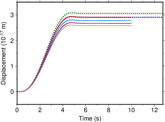
図1. 水平位置\((x,y)=(200,0)\)における\(x\)成分の変位波形。 実線はwaterPMLコマンドの結果であり、(0,0,-505)の位置にソースを置いたときの 地表下5 m(赤)、15 m(水色)、25 m(紫)、35 m(茶色)の計算結果を示す。 点線は波数積分法による地表での変位を示しており、 緑はソースを(0,0,-500)に置いた場合の結果、 青はソースを(0,0,-510)に置いた場合の結果である。
Fig. 1. Displacement waveforms (\(x\)-component) at a horizontal location \((x,y)=(200,0)\). Solid lines show the results from the waterPML command, where the source is located at (0,0,-505) and the station is located at 5 m (red), 15 m (light blue), 25 m (cyan), and 35 m (brown) below the ground surface. Dotted lines show the results from the discrete wavenumber method, where the station is located at the ground surface and the source is located at (0,0,-500) and (0,0,-510) in cases of the green and blue lines, respectively.