waterPMLコマンドの検証

1. 無限均質媒質中での計算

(Examples and validations for waterPML command — 1. computation in a homogeneous infinite medium)


◆概要とコマンド (Outline and the command)

waterPMLコマンドは複雑な地表面形状を考慮した波動場計算のためのプログラムであるが、 無限均質媒質中の波動場を計算することも可能であり、 プログラムの使い方の理解と計算コードの検証の最初の1歩として有用である。 Maeda et al. (2011)の3.1節において無限均質媒質中の波動場の計算例が示されており、 これを再現するためのコマンドは以下の通りである。
Although the purpose of the waterPML command is to compute a wavefied below a complicated surface topography, it can compute the wavefield in a homogeneous infinite medium. This is useful as the first step to understand the usage of the program and to checck the computation code. An example of such calculation is shown in Section 3.1 of Maeda et al. (2011) and can be reproduced by the command below.

waterPML --Nx=51 --Npmx=10 --x0=-510.0 --y0=-510.0 --z0=-510.0 --dx=20.0 --dt=0.002 --tmax=10.0 --structure_file=structure.ini --structure_file_format=layer --source_file=source.ini --output_dir=result01 --station_file=station_list.dat --snapshot_grid=specify:file=snapshot.ini --snapshot_dt=0.5

この例では--Nx=51 --dx=20.0のオプションにより 20 mサイズの格子セルを\(x\)方向に51個配置している。 したがって物理領域の\(x\)方向の長さは1020 mであり、 --x0=-510.0の指定と組み合わせることで \(-510 \leq x \leq 510\)(単位:m)と物理領域の座標範囲が決まる。
In this example, the options --Nx=51 and --dx=20.0 result in 51 grid cells of 20 m size (1020 m in total) in the physical volume along the \(x\)-direction. Combined with the --x0=-510.0 option, the coordinate range of the physical volume is determined as \(-510 \leq x \leq 510\) (unit: m).

Ny, Nzについては省略時はNxと同じになる。 またdy, dzについても省略時はdxと同じになる。 したがって上記のオプションでは物理領域の\(y\)方向、\(z\)方向の範囲も \(-510 \leq y,z \leq 510\)(単位:m)となる。
When omitted, the values of parameters Ny and Nz are equal to Nx and those of dy and dz are equal to dx. Therefore, the coordinate ranges of the physical volume along the \(y\)- and \(z\)-directions are \(-510 \leq y,z \leq 510\) (unit: m).

--Npmx=10のオプションにより PML領域の厚さを格子セル10個分(200 m)にしている。
The --Npmx=10 option results in 10 grid cells (200 m thickness) in the PML volume.

--dt=0.002 --tmax=10.0のオプションにより 0.002 sの時間刻みで10 sまでの波動場を計算することを指定している。 また、出力ファイルのサイズを抑えるため、 波動場のスナップショットは全ての時間ステップで出力するのではなく 0.5 s毎に出力する設定にしている(--snapshot_dt=0.5)。
The options --dt=0.002 and --tmax=10.0 result in the computation of the wave field until 10 s with a time stepping of 0.002 s. To save the output file size, the snapshots of the wave field are not written at every time step of the computation but are written at every 0.5 s (--snapshot_dt=0.5).

上記のコマンドでは--topography_filesオプションが省略されている。 したがって地表面無し(無限媒質)での計算となる。
A --topography_files option is omitted in the command above. Therefore the computation does not use a ground surface (i.e., a computation in an infinite medium).

上記のコマンドではいくつかの設定ファイルを参照しており、 これらを前もって作成しておく必要がある。 以下、設定ファイルの例示と説明である。
The command above refers to several configuration files, which must have been created in advance to the command run. Examples and descriptions for these configuration files are given below.


●地下構造 (A subsurface structure)

waterPMLコマンドでは地下構造は以下の2種類の方法で指定できる。
The waterPML command can specify the subsurface structure by one of the following ways.

無限媒質は一種の水平成層構造であるので、より簡単なlayerでの指定が可能である。 --structure_file=structure.ini --structure_file_format=layer のオプションは地下構造をstructure.iniという名前のファイルで与えること、 その書式がlayer用のものであることを示している。
Because a homogeneous medium is a kind of a stratified medium, it can be specified by the layer option that is easier than subdomain. The --structure_file=structure.ini and --structure_file_format=layer options indicate that the subsurface structure is given by a file named structure.ini and its format is based on layer.

以下がstructure.iniの例である。 物理領域の\(z\)座標の範囲が\(-510\leq z\leq 510\)であるのでこれをカバーするように、 またこの後の例題で\(z\geq -1000\)までの範囲を用いるのでそれもカバーするように、 \(-1100\leq z\leq 600\)の範囲での地下構造を与えている。 ここではP波速度\(V_p=2000\) m s\(^{-1}\)、 S波速度\(V_s=V_p/\sqrt{3}\sim 1154.7\) m s\(^{-1}\)、 密度2500 kg m\(^{-3}\) の均質媒質としている。
An example of structure.ini is shown below, which extends over \(-1100\leq z\leq 600\). This range was chosen to be wider than the \(z\)-coordinate range of the physical volume in this example (\(-510\leq z\leq 510\)) and later examples where \(z\geq -1000\) is used. A P-wave velocity \(V_p=2000\) m s\(^{-1}\), an S-wave velocity \(V_s=V_p/\sqrt{3}\sim 1154.7\) m s\(^{-1}\), and a density of 2500 kg m\(^{-3}\) are used.

(structure.ini)
600.0[TAB]2000.0[TAB]1154.7[TAB]2500.0
-1100.0[TAB]2000.0[TAB]1154.7[TAB]2500.0

ここで[TAB]はタブを表す (空白であってはならない)。
Here, [TAB] represents a tab (which must not be a space).

なおMaeda et al. (2011)ではS波速度として1100 m s\(^{-1}\)を使用した。 そのため厳密に\(V_s=V_p/\sqrt{3}\)にはなっておらず、 この例題で示す計算結果とは波形の振幅がややずれる。
Note that Maeda et al. (2011) used an S-wave velocity of 1100 m s\(^{-1}\), which does not exactly satisfy \(V_s=V_p/\sqrt{3}\). Therefore, the results shown in this page and Maeda et al. (2011) have slight differences in the amplitudes of waveforms.


●地震波動ソース (A seismic wave source)

ここではMaeda et al. (2011)の3.1節にならい、 1 N mのダイポールソース(\(x\)方向; \(M_{xx}\))を(0,0,0)の位置に与えることにする。 震源時間関数は \[\begin{equation} f(t)= \begin{cases} 0 & (t<0) \\ 10\left(\frac{t}{\tau_p}\right)^3 -15\left(\frac{t}{\tau_p}\right)^4 +6\left(\frac{t}{\tau_p}\right)^5 & (0\leq t \leq \tau_p) \\ 1 & (\tau_p<t) \end{cases} \label{eq.timefunc} \end{equation}\] とし、時定数を\(\tau_p=5\) sとする。 ymaeda_opentoolsにおいて(\ref{eq.timefunc})式の時間関数は pow5という関数名で定義されている。 したがって地震波動ソースの指定は以下のように書ける。
Following Section 3.1 of Maeda et al. (2011), a dipole source of 1 N m along the \(x\)-direction (\(M_{xx}\)) is applied at a location of (0,0,0). The source time function is given by Eq. (\ref{eq.timefunc}) with a time constant \(\tau_p=5\) s. In ymaeda_opentools, a time function of Eq. (\ref{eq.timefunc}) is available with a function name pow5. Therefore, the configuration of the seismic wave source is given as below.

(source.ini)
newsource dipole
location_x=0.0
location_y=0.0
location_z=0.0
mechanism=Mxx
intensity=1.0
stfun_name=pow5
stfun_tp=5.0

このファイルはwaterPMLコマンドの--source_file=source.iniオプションによって 計算に取り込まれる。
This file is incorporated into the computation by the --source_file=source.ini option of the waterPML command.

物理領域の範囲を\(-500\leq x\leq 500\)ではなく \(-510\leq x\leq 510\)としたのは (0,0,0)の位置に地震波動ソースを置くためである。 地震波動ソースは格子セル中心点で近似されるので、 もし物理領域を\(-500\leq x\leq 500\)とすると\(x=0\)が格子セルの境界になってしまい、 地震波動ソースの位置が\(x=10\)または\(x=-10\)にずれてしまう。 \(y\), \(z\)についても同様である。
The purpose of the choice of the physical volume (not \(-500\leq x\leq 500\) but \(-510\leq x\leq 510\)) is to place the seismic wave source exactly at (0,0,0). The seismic wave source location is approximated at the center of a grid cell. If the physical volume was \(-500\leq x\leq 500\), \(x=0\) would be a boundary between grid cells, and the source location would deviate to \(x=10\) or \(x=-10\). The same argument is applied to \(y\) and \(z\).


●観測点 (Stations)

Maeda et al. (2011)の図4では計算結果を (100,0,0), (200,0,0), (400,0,0), (200,200,0) の4地点で示している。 そこで、これら4地点に観測点を置くことにする。
Fig. 4 of Maeda et al. (2011) shows the computation results at four points (100,0,0), (200,0,0), (400,0,0), and (200,200,0). To output the waveforms at these locations, stations are placed there.

(station_list.dat)
station_a[TAB]100.0[TAB]0.0[TAB]0.0
station_b[TAB]200.0[TAB]0.0[TAB]0.0
station_c[TAB]400.0[TAB]0.0[TAB]0.0
station_d[TAB]200.0[TAB]200.0[TAB]0.0

このファイルはwaterPMLコマンドの--station_file=station_list.datオプションによって 計算に取り込まれる。
This file is incorporated into the computation by the --station_file=station_list.dat option of the waterPML command.


●スナップショットの設定 (Configuration of snapshots)

Maeda et al. (2011)の図3では \(z=0\)の断面上で波動場のスナップショットを表示している。 同様のスナップショットを得るため、waterPMLコマンドに --snapshot_grid=specify:file=snapshot.ini オプションを渡し、このsnapshot.iniを以下のように記載する。
Fig. 3 of Maeda et al. (2011) shows the snapshots of the wave field on a section of \(z=0\). To obtain the same snapshot data, a --snapshot_grid=specify:file=snapshot.ini option is given to the waterPML command, and the file snapshot.ini is written as below.

(snapshot.ini)
newsnap z0
snapname z0
xrange -700.0,700.0
yrange -700.0,700.0
zrange -1.0,1.0

ここではPML領域を含めた計算領域全体でのスナップショットを得るために \(x\), \(y\)座標の範囲を\(-700\leq x,y\leq 700\)としている。 また\(z=0\)での断面を得るために\(-1\leq z\leq 1\)としている。 格子セル中心点での計算結果が出力されるので、\(z\)座標の範囲をこのようにすれば \(z=0\)での値のみが出力される。
Here, the coordinate ranges for \(x\) and \(y\) are given as \(-700\leq x,y\leq 700\) to obtain the snapshots over the entire computational volume, including the PML volume. The range of \(z\) is specified as \(-1\leq z\leq 1\) to obtain a section on \(z=0\). Because the computation results are written at the centers of grid cells, this range of \(z\) results in outputting the values only at \(z=0\).


◆スナップショットの確認 (Checking the snapshots)

上記のコマンドを実行するとresult01ディレクトリが作成され、その下に
が作成される。このうちsnapshotサブディレクトリ内に 波動場のスナップショット(\(z=0\)の断面)が出力される。
When you execute the command above, a directory result01 is created, which consist of:
The snapshots of the wavefield on a section of \(z=0\) are available in the snapshot subdirectory.

ここでは例として時刻\(t=1.5\) sでの速度場の\(x\)成分のスナップショットを見てみることにする。 このデータは上記ディレクトリの下、z0.Vx.t1.5000.3dbというファイルに格納されている。 z0はsnapshot.iniで指定したスナップショットの名前、Vxは速度場の成分、t1.5000は時刻を表す。 拡張子の.3dbはこのデータが ymaeda_opentoolsの3次元データファイル形式 の1つである 3db形式 で書かれていることを表している。 このままではバイナリファイルであり中身を見られないので、 3d_data_convertコマンド を用いてテキストファイル (3d形式) に変換する。 コマンド例を以下に示す。
Now, let us look at the snapshot of the velocity field of \(x\)-component at time \(t=1.5\) s. This data is stored in a file z0.Vx.t1.5000.3db in the directory described above, where z0 is the name of the snapshot specified in snapshot.ini, Vx represents the component of the velocity field, and t1.5000 represents time. The extension .3db indicates that this file is written with a 3db format, which is one of the file formats for 3-D data in ymaeda_opentools. Because it is a binary file that cannot directly be shown, let us convert to a text file (3d format) using 3d_data_convert command, as shown below.

cd result01/snapshot
3d_data_convert z0.Vx.t1.5000 3db 3d

これにより、z0.Vx.t1.5000.3dというテキストファイルが作成される。 その第1列は\(x\)座標(単位:m)、第2列は\(y\)座標、第3列は\(z\)座標(今回の例では全て0)、 第4列は速度の\(x\)成分\(V_x\)の値(単位:m/s)を表す。
By this, a text file z0.Vx.t1.5000.3d is created. The 1st column of this file represents a \(x\)-coordinate (unit: m), tne 2nd does \(y\), and the 3rd does \(z\) that is all zero in this example. In the 4th column, the \(x\)-component of the velocity \(V_x\) (unit: m/s) is written.

ymaeda_opentoolsには計算結果のプロットのためのツールは用意していないが、 このような形式のテキストファイルが得られれば 一般的な描画ツールを用いてプロットするのは容易である。例えばawkと Generic Mapping Tools (version 6) を組合せて以下のようにプロットできる。
Although ymaeda_opentools does not consist of tools to plot the computation results, it is easy to plot the data in the text file of this format using general plotting tools. For example, the data can be plotted with the commands below, where awk and Generic Mapping Tools (version 6) are combined.

gmt begin z0.Vx.t1.5000 ps

gmt set FONT_ANNOT_PRIMARY 12p

awk 'BEGIN{ FS="\t" }(NF==4){ print $1,$2,$4*1e+17 }' z0.Vx.t1.5000.3d | gmt xyz2grd -R-700/700/-700/700 -I20/20 -Gz0.Vx.t1.5000.grd

gmt makecpt -Cpolar -T-5/5/0.1 -Z -D

gmt grdimage z0.Vx.t1.5000.grd -R-700/700/-700/700 -JX7/7 -Xa2 -Ya5 -Bxa500f100 -Bya500f100 -BWSen

gmt colorbar -Dx5.5/4/4/0.5h -Bxa2f1 -BS

gmt text -R0/21/0/29.7 -JX21/29.7 -Xa0 -Ya0 -F+f12p+jCT <<EOF
5.5 2.7 Velocity Vx (10@+-17@+ m/s)
EOF

gmt end

これにより、z0.Vx.t1.5000.psという画像ファイルが作成される。 図1にこの画像を示す。 (0,0,0)の位置に\(x\)軸方向のダイポールソース(\(M_{xx}\))を置いたのであるから \(V_x\)は\(x=0\)に関して反対称な分布になることが期待され、 実際にその通りの分布になっていることが分かる。 また、物理領域は\(-510\leq x,y\leq 510\)の範囲であり、 その外側はPML領域である。 PML領域内で波動が吸収されていることも図1から見て取れる。 以上の特徴より妥当な波動場が得られたと判断できる。 より多くの時刻で同様の検証を行った結果が Maeda et al. (2011)の3.1節および図3に示されている。
By this, an image file z0.Vx.t1.5000.ps is created, which is shown in Fig. 1. Because a dipole source along the \(x\)-direction (\(M_{xx}\)) was applied at (0,0,0), \(V_x\) is expected to be anti-symmetric with respect to \(x=0\). Fig. 1 is consistent with this expected spatial distribution of \(V_x\). In addition, Fig. 1 shows that the wave is absorbed in the PML volume that is outside of the physical volume in \(-510\leq x,y\leq 510\). These characteristics suggest the validity of the wave field computed. Section 3.1 and Fig. 3 of Maeda et al. (2011) show the results of similar validation to different time steps.


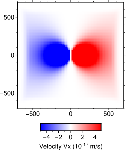
図1. 時刻\(t=1.5\) sでの速度の\(x\)成分\(V_x\)のスナップショット。
Fig. 1. A snapshot of the \(x\)-component velocity \(V_x\) at time \(t=1.5\) s.


◆波形の確認 (Checking the waveforms)

無限均質媒質中の計算を行う利点は解析解との比較による検証が可能なことである。 ymaeda_opentoolsでは WIHMコマンド を用いて解析解の計算を行うことができる。 以下ではwaterPMLコマンドとWIHMコマンドで得られた波形の比較を行う。
The purpose of the computation in the infinite homogeneous medium is to check the results by comparison with an analytical solution. In ymaeda_opentools, WIHM command is available to compute the analytical solution. Below, a comparison of the waveforms obtained by waterPML and WIHM commands is shown.


●WIHMコマンドによる解析解の計算 (Computation of an analytical solution using WIHM command)

Maeda et al. (2011)の図4で示した4地点のうち、 ここでは例として(200,0,0)の位置での解析解を計算する。
Let us compute the analytical solution at a location (200,0,0) as an example. This is one of the four points shown in Fig. 4 of Maeda et al. (2011).

WIHM --tmax=10.0 --dt=0.002 --Vp=2000.0 --Vs=1154.7 --rho=2500.0 --source_file=source.ini --station_name=station_b --station_location=200,0,0 --outputfile=result01_WIHM/station_b

これにより、result01_WIHMディレクトリの下に以下の3つのファイルが作られる。
This command creates the following three files under result01_WIHM directory.


以下では\(x\)成分についてwaterPMLコマンドの結果と比較する。 seq1形式 ymaeda_opentoolsの時系列データファイル形式 の1つであるが、各時刻での変位の値のみが書かれているのでこのままではプロットしづらい。 そこで sequencefile_convertコマンド を用いて時刻と変位の値の組のデータ (seq2形式) に変換する。
Below the \(x\)-component is compared with that from the waterPML command. The seq1 format is one of the file formats for time series data in ymaeda_opentools and consists only of the value of displacement at each sample. It is not easy to plot. Therefore, let us convert the data to a combination of time and displacement values ( seq2 format) using sequencefile_convert command.

cd result01_WIHM
sequencefile_convert station_b.Ux seq1 seq2
cd ..

これによりresult01_WIHMディレクトリの下にファイルstation_b.Ux.seq2が作られる。 これは位置(200,0,0)における\(x\)成分の変位波形を表しており、 最初の4行はヘッダで5行目以降は第1列が時刻(s)、第2列が変位(m)である。
By this, a file station_b.Ux.seq2 is created under the directory result01_WIHM. It represents an \(x\)-component displacement waveform at the location (200,0,0). The 1st to 4th lines in this file are headers, and the data after 5th lines are written with the time (s) in the 1st column and displacement (m) in the 2nd column.

他の地点での波形も同様に計算できる。 なおWIHMコマンドでは1度の計算では1つの観測点の波形しか計算できないので、 4地点で波形を計算するには単純にWIHMコマンドを4回実行する。
The waveforms at other locations can be computed in the same way. Note that a single run of the WIHM command computes the analytical solution at one site. Therefore, to compute the waveforms at the four points, simply repeat the WIHM command four times.


●waterPMLコマンドによる計算結果の整形 (Arranging the computation results of waterPML command)

waterPMLコマンドで計算した波形はresult01/waveformディレクトリに格納されている。 (200,0,0)の位置における\(x\)成分の速度波形データは 上記ディレクトリ内のstation_b.Vx.seq1に書かれている。 seq1形式をseq2形式に変換することに加え、 WIHMコマンドで求めた解析解との比較のために変位波形に直す必要がある。 速度波形から変位波形への換算にはymaeda_opentoolsの sequencefile_integralコマンド が利用できる。 以下がコマンド例である。
The waveforms computed by the waterPML command are stored in result01/waveform directory. The \(x\)-component velocity waveform data at the location (200,0,0) is written in a file station_b.Vx.seq1 under this directory. In addition to the format conversion from seq1 to seq2, the velocity waveform must be transformed to displacement to compare it with the analytical solution derived by the WIHM command. In ymaeda_opentools, sequencefile_integral command is available to transform a velocity waveform to displacement, as shown below.

cd result01/waveform
sequencefile_integral station_b.Vx.seq1 station_b.Ux.seq2
cd ../..


●波形の比較 (Comparison of the waveforms)

以上でwaterPMLコマンド(数値解)とWIHMコマンド(解析解)による 同じ地点(200,0,0)での同じ\(x\)成分の変位波形の数値データが得られたので、 これらを重ねてプロットすることで数値解の精度を評価できる。 Generic Mapping Tools (version 6) を用いたプロットの例を以下に示す。
Numerical data for displacement waveforms at the same location (200,0,0) and the same \(x\)-component from waterPML (numerical) and WIHM (analytical) have been obtained. Plotting them together, we can examine the accuracy of the numerical solution. An example of the plotting commands is shown below, where Generic Mapping Tools (version 6) is used.

mkdir result01_waveform_comparison

cd result01_waveform_comparison

gmt begin station_b.Ux ps

gmt set FONT_ANNOT_PRIMARY 12p

awk '(NF==2){ print $1,$2*1e+16 }' ../result01_WIHM/station_b.Ux.seq2 | gmt plot -R0/10/-0.5/7 -JX10/7 -Xa3 -Ya3 -W2,0/127/255

awk '(NF==2){ print $1,$2*1e+16 }' ../result01/waveform/station_b.Ux.seq2 | gmt plot -R0/10/-0.5/7 -JX10/7 -Xa3 -Ya3 -W1,255/0/0 -Bxa2f1 -Bya2f1 -BWSen

gmt text -R0/21/0/29.7 -JX21/29.7 -Xa0 -Ya0 -F+f12p+a+j <<EOF
8 2.2 0 CT Time (s)
2.2 6.5 90 CB Displacement (10@+-16@+ m)
EOF

gmt end

得られた波形の比較図を図2に示す。 waterPMLコマンドの結果(数値解)を赤で、 WIHMコマンドの結果(解析解)を青で示している。 この図はMaeda et al. (2011)の図4bに対応する (但し、Maeda et al. (2011)ではS波速度を1100 m/sとしたのに対し、 この例題では1154.7 m/sとしている)。 数値解と解析解はよく合っており、 振幅の僅かなずれは地震波動ソースと観測点の間の格子セル数が 不足していることによると思われる (Maeda et al. (2011)の3.1節)。
The figure plotted by these commands is shown in Fig. 2. The red and blue line show waterPML (numerical) and WIHM (analytical) solutions, respectively. This figure corresponds to Fig. 4b of Maeda et al. (2011) except for the slight difference in the S-wave velocity explained earlier (1100 m/s in Maeda et al. (2011) and 1154.7 m/s in this page). The numerical and analytical solutions are well fitted. A slight difference in the amplitude is likely caused by an insufficient number of grid cells between the seismic wave source and the station (Section 3.1 of Maeda et al. (2011)).


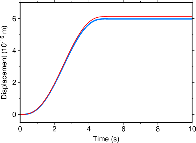
図2. 位置(200,0,0)における\(x\)成分の変位波形。 赤:waterPMLコマンドの結果(数値解)、 青:WIHMコマンドの結果(解析解)。
Fig. 2. Displacement waveforms (\(x\)-component) at a location (200,0,0). Red and blue lines show waterPML (numerical) and WIHM (analytical) solutions, respectively.