winvコマンドマニュアル 例題

2. 直交座標の計算

(A practice for winv command step 2; calculating cartesian coordinates)


2-1. 直交座標が必要になる理由 (Reasons that cartesian coordinates are needed)

観測点の座標は通常、緯度経度で与えられる。 今回の例題でもステップ1で見たように 緯度経度で与えられている。 また地形データについても緯度経度で与えられている。 実際の解析においても、 例えば国土地理院が発行している基盤地図情報の数値標高モデルを用いる場合には 緯度経度ベースのデータとなる。
Station coordinates are usually given by latitudes and longitudes. This is true in this exercise, as we have seen in step 1. Topography data is also given based on latitudes and longitudes. In real data analysis, if you use a digital elevation model in a basis map information issued by the Geospatial Information Authority of Japan, it is given based on latitudes and longitudes.

winvコマンドでは観測点の座標や地形データは直接には使用しない。 しかし実用グリーン関数を waterPMLコマンド を用いて計算することを想定している。 waterPMLコマンドでは計算の単純化のため直交座標系を用いており、 ソースや観測点の位置を直交座標で表現する。
The winv command does not directly use station coordinates and topography data. However, practical Green’ functions are supposed to be computed by waterPML command, which uses a cartesian coordinate system for simplicity of computations and thus expresses source and station locations by the cartesian coordinates.

またwinvコマンドにおいてもソース位置の表現に直交座標が用いられる。 ソース位置の探索範囲を検討する上でも観測点の直交座標を知っておくことが望ましい。
In addition, the winv command expresses a source location by a cartesian coordinate. Knowing the cartesian coordinates of stations would help consideration of an appropriate search range of the source location.

このような理由から直交座標が必要になる。
For these reasons, cartesian coordinates are needed.


2-2. 直交座標系の基準点の決定 (Determining the reference point of the cartesian coordinate system to use)

直交座標系とは本来は球面である地表面を 狭い空間範囲において平面で近似したものである。 この近似には基準点が必要である。 解析の対象領域と基準点が離れていると近似による誤差が大きくなるので 基準点は解析領域内に取るのが良い。 火山地域を対象とする解析の場合、 対象とする火山の山頂あるいは噴火口の中心点を基準点に取ると分かりやすい。
A cartesian coordinate system is an approximation of a spherical ground surface by a flat plane in a narrow spatial range. This approximation requires a reference point. An error in the flat plane approximation would be minimized by taking the reference point in the target region of the analysis. In case of analyses in volcanic fields, a good choice for the reference point would be the summit or the center of an eruptive crate of the volcano.

今回は山頂を基準点に取ることにする。 山頂は最も標高が高い場所であるので地形データをソートすることで位置を調べられる。 例えば以下のコマンドで山頂の緯度経度が分かる。
In this exercise, let us use the summit as the reference point. The summit is the highest location of the ground surface elevation and can be surveyed by sorting topography data. The command below returns the latitude and longitude of the summit.

sort -gr +2.0 -3.0 topography.dat | head

このコマンドではファイルtopography.datのデータを第3列の値に基づいて降順にソートして 最初の数行を画面に表示する。 コマンドを実行した結果を以下に示す。
This command sorts the data in file topography.dat in a descending order based on the values in the 3rd column and displays the first several lines. The result is shown below.

34:22:40    137:12:34    2988.0
34:22:38    137:12:34    2988.0
34:22:38    137:12:36    2979.1
34:22:40    137:12:36    2978.6
34:22:42    137:12:34    2975.6
34:22:36    137:12:34    2972.7
34:22:42    137:12:36    2966.0
34:22:36    137:12:36    2964.3
34:22:44    137:12:34    2956.1
34:22:44    137:12:36    2946.3

この結果から
(1)北緯34度22分40秒、東経137度12分34秒
(2)北緯34度22分38秒、東経137度12分34秒
の2つの格子点(2秒刻みの地形データであるのでこれらは隣接している) において標高は最大値2988mとなっている。 その間を取った 北緯34度22分39秒、東経137度12分34秒 を直交座標の基準点として用いることにする。
This result shows that the ground surface elevation is maximal (2988 m) at two grid nodes:
(1) 34°22’40”N, 137°12’34”, and
(2) 34°22’38”N, 137°12’34”.
These two grid nodes are adjacent because the topography data is given at 2-s intervals. Taking the average of them, we hereafter use 34°22’39”N, 137°12’34” as the reference point of the cartesian coordinate system in this exercise.


2-3. 観測点の直交座標の計算 (Calculating the cartesian coordinates of stations)

緯度経度から直交座標への変換にはymaeda_opentoolsの latlon2xyコマンド が使用できる。 例えばファイルstations_latlon.datにおいて観測点NU.N01の座標は 北緯34.3840度、東経137.2080度と与えられている。 これを直交座標に変換するには以下のコマンドを実行すれば良い。
Users can use latlon2xy command of ymaeda_opentools to compute a cartesian coordinate from a latitude and a longitude. For example, the coordinate of station NU.N01 is given as 34.3840°N, 137.2080°E in file stations_latlon.dat. The corresponding cartesian coordinate can be computed by the command shown below.

latlon2xy --N=34.3840 --E=137.2080 --refN=34:22:39 --refE=137:12:34

ここで基準点の座標(--refN, --refEオプション)には 2-2節で調査した山頂の座標を用いている。 コマンドを実行すると以下のように表示される。
Here, the coordinate of the summit surveyed in Section 2-2 is used for the reference point (--refN and --refE options). The command outputs the following results in the display.

-132.8279    720.9692

この1つ目の値(-132.8279)が観測点NU.N01の\(x\)座標(基準点から東方向、m)、 2つ目の値(720.9692)が\(y\)座標(基準点から北方向、m)である。
The 1st value (-132.8279) is an \(x\)-coordinate (east from the reference point, m) and the 2nd value (720.9692) is a \(y\)-coordinate (north from the reference point, m) of the station NU.N01.


2-3-1. 全観測点の座標の一括変換 (Calculating the cartesian coordinates of all stations at once)

観測点数が多い場合、このように1つずつ変換するよりも 全ての観測点の座標を一括で変換する方が早いしミスも起きにくい。 latlon2xyコマンドを用いて複数の座標を一括変換するにはまず 第1列を緯度、第2列を経度、第3列をその他の情報とするファイルを作成する必要があり、 今回の例では以下のコマンドで作成できる。
If a lot of stations are available, converting the coordinates of all stations at once is faster and more free from mistakes than one-by-one conversions. The conversion at one requires a file in which the 1st column shows latitudes, the 2nd column does longitudes, and 3rd does the other information. This file can be created by the command below in this example.

awk '{ printf("%f\t%f\t%s\n",$2,$3,$1) }' stations_latlon.dat > tmp1.dat

ここでは列の区切り文字が確実にタブになるように書式指定をしている (スペースが区切り文字になってしまうと次のステップでエラーになる)。
Note that the output format is specified to separate the columns by tabs; if spaces are used as the separaters, the next step would fail.

次に、作成されたファイル(tmp1.dat)を入力としてlatlon2xyコマンドを実行する。
Next, execute latlon2xy command using the file created in the previous step (tmp1.dat) as the input.

latlon2xy --inputfile=tmp1.dat --outputfile=tmp2.dat --refN=34:22:39 --refE=137:12:34

作成されるファイル(tmp2.dat)は第1列が\(x\)、第2列が\(y\)、第3列がその他の情報 (今回の場合は観測点コード)になっている。 このままでも良いがstations_latlon.datに合わせて第1列が観測点コードになるように整形する。
The file created by this step (tmp2.dat) consists of \(x\)-coordinates in the 1st column, \(y\)-coordinates in the 2nd column, and the other information (station codes in this case) in the 3rd column. Let us move the station code to the 1st column for consistency with stations_latlon.dat (although this is not mandatory).

awk '{ printf("%s\t%f\t%f\n",$3,$1,$2) }' tmp2.dat > stations_xy.dat

こうして stations_xy.dat が作成されたらtmp1.dat, tmp2.datは削除して構わない。
You can remove tmp1.dat and tmp2.dat once stations_xy.dat was created.


2-4. 直交座標系で表現された地形データの作成 (Creating a topography data in the cartesian coordinate system)

waterPMLコマンドには緯度経度で表現された地形データを直接読み込む機能があり、 winvコマンドでは地形データを直接には利用しない。 したがって地形データの直交座標への変換はプログラムを動かす上で必須ではない。 しかしソース位置の探索範囲の検討や、逆解析が終わった後で結果を地図にプロットする際などに 直交座標系で表現された地形データがあると便利である。 直交座標系で表現された地形データは以下のコマンドで作成できる。
Conversion of topography data to a cartesian coordinate system is not mandatory because waterPML command can directly read topography data on the latitudes and longitudes, and winv command does not directly use topography data. However, the topography data in the cartesian coordinate system is convenient when you consider a search range of the source location, or when you plot the waveform inversion results on a map. The cartesian-based topography data can be created by the command below.

latlon2xy --inputfile=topography.dat --outputfile=topography_xy.dat --refN=34:22:39 --refE=137:12:34


2-5. 直交座標系による地形と観測点のプロット (Plotting the topography and stations on the cartesian coordinate system)

直交座標系で表現された観測点リスト (stations_xy.dat; 2-3-1節で作成) と地形データ (topography_xy.dat; 2-4節で作成) を地図上にプロットしてみることも必須ではないがソース位置の探索範囲を検討する上で有益である。 どちらもテキストファイルであるのでユーザが使い慣れたツールを用いてプロットすれば良い (ymaeda_opentoolsにはプロット用のツールは無い)。 以下は Generic Mapping Tools (version 6.3.0) を用いてプロットするbashスクリプトの例である。
Plotting the data of stations (stations_xy.dat; created in Section 2-3-1) and topography (topography_xy.dat; created in Section 2-4) expressed in the cartesian coordinate system onto a map is not mandatory but useful when you determine a search range of the source location. Because the both files are text files, you can use any tools that you are familier for the plotting; there is no plotting tool in ymaeda_opentools. Below, a bash script with Generic Mapping Tools (version 6.3.0) to plot the data on a map is shown as an example.

#! /bin/bash -u

# 横軸の設定 (Configuration of the lateral axis)
xmin=`gmt info -C topography_xy.dat | awk '{ printf("%.2f",$1/1000.0) }'`
xmax=`gmt info -C topography_xy.dat | awk '{ printf("%.2f",$2/1000.0) }'`
xtics=1
mini_xtics=0.5

# 縦軸の設定 (Configuration of the vertical axis)
ymin=`gmt info -C topography_xy.dat | awk '{ printf("%.2f",$3/1000.0) }'`
ymax=`gmt info -C topography_xy.dat | awk '{ printf("%.2f",$4/1000.0) }'`
ytics=1
mini_ytics=0.5

# 標高の設定 (Configuration of the elevation)
zmin=1000.0
zmax=3100.0
zinc=1.0
ztics=1000.0
mini_ztics=500.0

# グラフのプロット位置とサイズの設定 (Configuration of the plotting location and size)
x0=3.0
y0=3.0
width=8.0
height=`echo $width $xmin $xmax $ymin $ymax | awk '{ print $1*($5-$4)/($3-$2) }'`
# カラーバーの設定 (Configuration of the color bar)
colorbar_x=`echo $x0 $width | awk '{ print $1+$2+0.5 }'`
colorbar_y=`echo $y0 $height | awk '{ print $1+$2/2.0 }'`
colorbar_length=`echo $height | awk '{ print 0.7*$1 }'`

# 出力ファイル名 (The output file name)
outputfile_noExt=map_xy

# プロットの開始 (Start plotting)
gmt begin $outputfile_noExt ps

# 座標軸の文字サイズを設定 (Set font size for coordinate axes)
gmt set FONT_ANNOT_PRIMARY 10p

# 地形データをgrdファイルに変換 (Convert the topography data to a grd format)
awk '{ print $1/1000.0,$2/1000.0,$3 }' topography_xy.dat | gmt surface -R${xmin}/${xmax}/${ymin}/${ymax} -Gtopography_xy.grd -I0.01/0.01

# カラーパレットの作成 (Create a color pallete)
gmt makecpt -Cdem1 -T${zmin}/${zmax}/${zinc} -Z

# 地形を色で表現 (Plot the topography by colors)
gmt grdimage topography_xy.grd -R${xmin}/${xmax}/${ymin}/${ymax} -JX${width}/${height} -Xa${x0} -Ya${y0}

# カラーバーのプロット (Plot a colorbar)
gmt colorbar -Dx${colorbar_x}/${colorbar_y}/${colorbar_length}/0.2 -Bxa${ztics}f${mini_ztics}

# カラーバーのレジェンドのプロット (Plot a colorbar legend)
echo ${colorbar_x} ${colorbar_y} | awk '{ print $1+1.4,$2,"Elevation (m)" }' | gmt text -R0/21/0/29.7 -JX21/29.7 -Xa0 -Ya0 -F+f10p+a270+jCB

# 細い等高線(100 m間隔)をプロット (Plot thin topography contours at 100 m intervals)
gmt grdcontour topography_xy.grd -R${xmin}/${xmax}/${ymin}/${ymax} -JX${width}/${height} -Xa${x0} -Ya${y0} -C100 -W0.4,200/150/100

# 太い等高線(500 m間隔)をプロット (Plot thick topography contours at 500 m intervals)
gmt grdcontour topography_xy.grd -R${xmin}/${xmax}/${ymin}/${ymax} -JX${width}/${height} -Xa${x0} -Ya${y0} -C500 -W1.2,200/150/100

# 観測点位置を記号でプロット (Plot station locations by stations)
awk '{ print $2/1000.0,$3/1000.0 }' stations_xy.dat | gmt plot -R${xmin}/${xmax}/${ymin}/${ymax} -JX${width}/${height} -Xa${x0} -Ya${y0} -St0.3 -G0/0/0

# 観測点コードをプロット (Plot station codes)
awk '{ print $2/1000.0,$3/1000.0-0.1,$1 }' stations_xy.dat | gmt text -R${xmin}/${xmax}/${ymin}/${ymax} -JX${width}/${height} -Xa${x0} -Ya${y0} -F+f10p+jCT -Bxa${xtics}f${mini_xtics} -Bya${ytics}f${mini_ytics} -BWSen

# 座標軸のレジェンドをプロット (Plot coordinate axis legends)
xlabel_x=`echo $x0 $width | awk '{ print $1+$2/2.0 }'`
xlabel_y=`echo $y0 | awk '{ print $1-0.6 }'`
ylabel_x=`echo $x0 | awk '{ print $1-0.8 }'`
ylabel_y=`echo $y0 $height | awk '{ print $1+$2/2.0 }'`
gmt text -R0/21/0/29.7 -JX21/29.7 -Xa0 -Ya0 -F+f10p+a+j <<EOF
$xlabel_x $xlabel_y 0 CT East (km) from the summit
$ylabel_x $ylabel_y 90 CB North (km) from the summit
EOF

# プロットの終了 (Finish the plotting)
gmt end

# png形式に変換 (Convert to a png format)
convert -trim -density 150 $outputfile_noExt.ps $outputfile_noExt.png

このスクリプトを実行すると下記の図2-1が作成される。 座標系を変換しただけであるので形は 図1-1と変わらない。 しかし例えば
というように距離感が一目瞭然になる。
Executing this script results in Fig. 2-1, which shows the same geometry as Fig. 1-1 because essentially the same data are plotted with only a conversion of coordinates. However, Fig. 2-1 gives more intuitive information for the distances, for example:


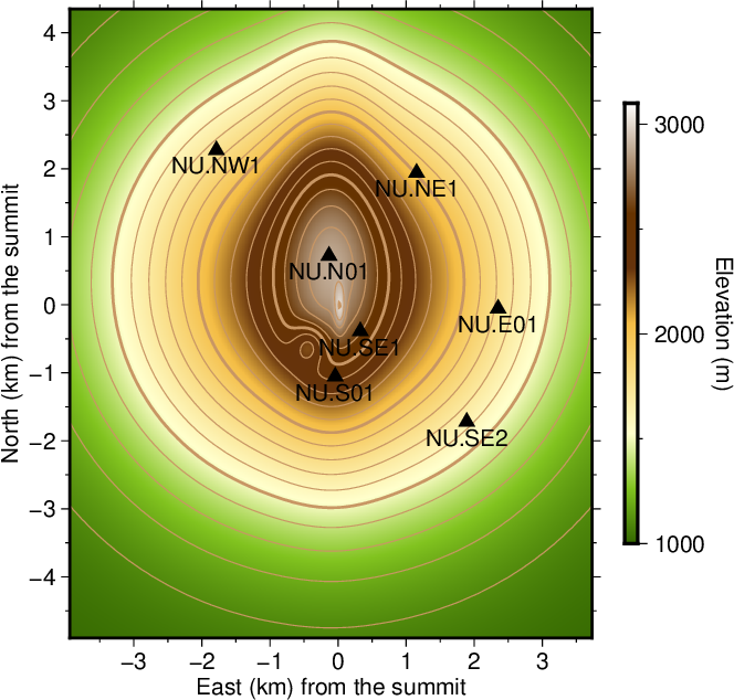
図2-1. 直交座標系による地形と観測点のプロット。
Fig. 2-1. A map of the topography and stations on a cartesian coordinate system.