winvコマンドマニュアル 例題

1. 練習用の架空のデータセットのダウンロードと確認

(A practice for winv command step 1; downloading and understanding a virtual dataset for practice)


1-1. データのダウンロード (Downloading data)

練習用の架空のデータセット一式は こちらのリンク からダウンロードできる。
Download a full set of virtual data from this link.

ファイル名は winv_exercise.tar.gz になっており、これを作業用のディレクトリに置いて以下のコマンドで解凍する。
The name of the file is winv_exercise.tar.gz. Place it in a working directory and uncompress by the command below.

tar xvfz winv_exercise.tar.gz

解凍すると winv_exercise というディレクトリが作成される。 以降の作業は全てこのディレクトリの下で行う。
By this, a directory winv_exercise is created. Perform all works below under this directory.


1-2. 観測点の座標 (Station coordinates)

この練習で使用する架空の観測点の座標は ダウンロードしたデータのディレクトリ(winv_exercise)の下の stations_latlon.dat というファイルに書かれている。 第1列が観測点コード、第2列が緯度(度)、第3列が経度(度)である。 観測点は全部で7観測点である。
The coordinates of virtual stations for this practice are available from a file stations_latlon.dat under the directory prepared above (winv_exercise). The 1st column of each line of the file indicates a station code, the 2nd column does the latitude (deg), and the 3rd does the longitude (deg) of the station. The number of stations is 7.


1-3. 地形データ (Topography data)

この練習で使用する架空の地形データ(数値標高モデル)は ダウンロードしたデータのディレクトリ(winv_exercise)の下の topography.dat というファイルで与えられる。 緯度経度の2秒刻みの格子点での地表面の標高のリストになっており、 第1列が緯度、第2列が経度(「度:分:秒」表記)、第3列が標高(m)である。
The topography data (a digital elevation model) for this practice is available from a file topography.dat under the directory prepared above (winv_exercise). This file gives the ground surface elevation on every grid node at 2-sec intervals along the latitude and longitude. The 1st column of each line represents the latitude, the 2nd column does the longitude (in “degree:minute:second” format), and the 3rd does the elevation (m).

この架空の地形データは北緯34度20-25分、東経137度10-15分の範囲をカバーしており、 1-2で述べた観測点は全てこの領域内にある。 実際にはこの領域は海域であるが、 topography.datで与えられる地形を持つ陸地であるものとして解析を行う (あくまで架空のデータである点を強調するためにあえて海域に架空の陸地を設定した)。
This virtual topography data extends over a spatial range of 34°20-25’N and 137°10-15’E, and all stations described in Section 1-2 are in this region. This region is actually in the sea; however, the analysis below assumes that this region is on the land with a topography given by this file. The sea region was chosen to prevent the readers from confusing the virtual topography and stations with actual ones.

逆解析を行う上で必須ではないが、 地形と観測点を地図にプロットしてみることは有益であろう。 ymaeda_opentoolsではプロット用のツールは用意していない。 観測点座標も地形データもテキストファイルであるので ユーザが使い慣れたツールを用いてプロットすれば良い。 以下は Generic Mapping Tools (version 6.3.0) を用いてプロットするbashスクリプトの例である。
It is good to plot the topography and stations on a map, although this is not mandatory. The ymaeda_opentools does not include tools for plottings; instead, users can use any other tools for plotting that they are familier, because the station coordinates and the topography are given by simple text files. Below, a bash script with Generic Mapping Tools (version 6.3.0) to plot the data on a map is shown as an example.

#! /bin/bash -u

# 横軸の設定 (Configuration of the lateral axis)
Emin=137:10:00
Emax=137:15:00
Etics=5m
mini_Etics=1m

# 縦軸の設定 (Configuration of the vertical axis)
Nmin=34:20:00
Nmax=34:25:00
Ntics=5m
mini_Ntics=1m

# 標高の設定 (Configuration of the elevation)
zmin=1000.0
zmax=3100.0
zinc=1.0
ztics=1000.0
mini_ztics=500.0

# グラフのプロット位置とサイズの設定 (Configuration of the plotting location and size)
x0=3.0
y0=3.0
width=8.0

# カラーバーの設定 (Configuration of the color bar)
colorbar_x=`echo $x0 $width | awk '{ print $1+$2+0.5 }'`
colorbar_y=`echo $y0 $width | awk '{ print $1+$2/2.0 }'`
colorbar_length=`echo $width | awk '{ print 0.7*$1 }'`

# 出力ファイル名 (The output file name)
outputfile_noExt=map

# プロットの開始 (Start plotting)
gmt begin $outputfile_noExt ps

# 座標軸の文字サイズを設定 (Set font size for coordinate axes)
gmt set FONT_ANNOT_PRIMARY 10p

# 地形データをgrdファイルに変換 (Convert the topography data to a grd format)
awk '{ print $2,$1,$3 }' topography.dat | gmt surface -R${Emin}/${Emax}/${Nmin}/${Nmax} -Gtopography.grd -I2s/2s

# カラーパレットの作成 (Create a color pallete)
gmt makecpt -Cdem1 -T${zmin}/${zmax}/${zinc} -Z

# 地形を色で表現 (Plot the topography by colors)
gmt grdimage topography.grd -R${Emin}/${Emax}/${Nmin}/${Nmax} -JM${width} -Xa${x0} -Ya${y0}

# カラーバーのプロット (Plot a colorbar)
gmt colorbar -Dx${colorbar_x}/${colorbar_y}/${colorbar_length}/0.2 -Bxa${ztics}f${mini_ztics}

# カラーバーのレジェンドのプロット (Plot a colorbar legend)
echo ${colorbar_x} ${colorbar_y} | awk '{ print $1+1.4,$2,"Elevation (m)" }' | gmt text -R0/21/0/29.7 -JX21/29.7 -Xa0 -Ya0 -F+f10p+a270+jCB

# 細い等高線(100 m間隔)をプロット (Plot thin topography contours at 100 m intervals)
gmt grdcontour topography.grd -R${Emin}/${Emax}/${Nmin}/${Nmax} -JM${width} -Xa${x0} -Ya${y0} -C100 -W0.4,200/150/100

# 太い等高線(500 m間隔)をプロット (Plot thick topography contours at 500 m intervals)
gmt grdcontour topography.grd -R${Emin}/${Emax}/${Nmin}/${Nmax} -JM${width} -Xa${x0} -Ya${y0} -C500 -W1.2,200/150/100

# 観測点位置を記号でプロット (Plot station locations by stations)
awk '{ print $3,$2 }' stations_latlon.dat | gmt plot -R${Emin}/${Emax}/${Nmin}/${Nmax} -JM${width} -Xa${x0} -Ya${y0} -St0.3 -G0/0/0

# 観測点コードをプロット (Plot station codes)
awk '{ print $3,$2-0.001,$1 }' stations_latlon.dat | gmt text -R${Emin}/${Emax}/${Nmin}/${Nmax} -JM${width} -Xa${x0} -Ya${y0} -F+f10p+jCT -Bxa${Etics}f${mini_Etics} -Bya${Ntics}f${mini_Ntics} -BWSen

# プロットの終了 (Finish the plotting)
gmt end

# png形式に変換 (Convert to a png format)
convert -trim -density 150 $outputfile_noExt.ps $outputfile_noExt.png

このスクリプトではymaeda_opentoolsを用いていないので中身について解説はしない。 必要ならばGeneric Mapping Toolsのマニュアルを参照のこと。 上記のスクリプトを実行すると下記の図1-1が作成される。
I do not explain this script because it does not use ymaeda_opentools; see the documentation of Generic Mapping Tools, if necessary. Fig. 1-1 is the figure created by this script.


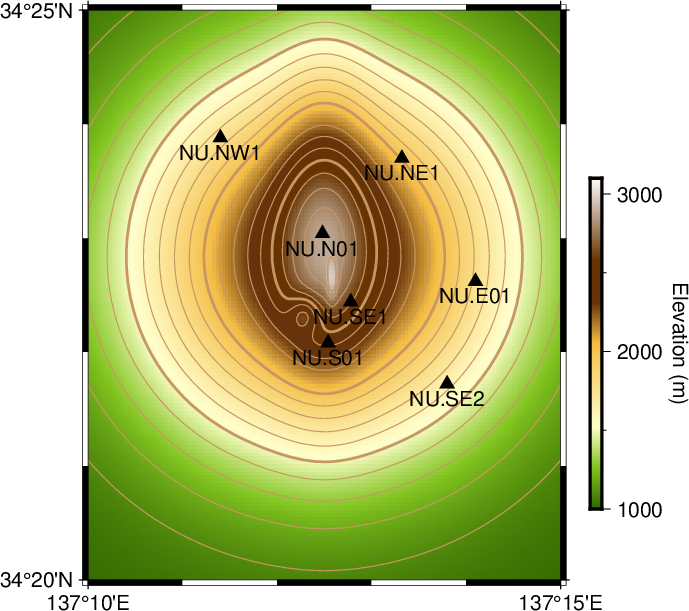
図1-1. 使用する架空の地形と観測点。
Fig. 1-1. The virtual topography and stations used.


1-4. 波形データ (Waveform data)

波形データはダウンロードしたディレクトリ(winv_exercise)の下の waveforms というサブディレクトリの下に 観測点コード.成分コード.sac の名前で格納されている。 観測点コードはファイルstations_latlon.dat(1-2節)に基づいており、 成分コードは東西がE(東向きが正)、南北がN(北向きが正)、上下がU(上向きが正)である。 例えばNU.SE2.N.sacは観測点NU.SE2の南北成分の波形である。
The waveform data are available with file names based on a rule station.component.sac, where station is the station code based on file stations_latlon.dat (Section 1-2) and component is E for east-west (positive: eastward), N for north-south (positive: northward), and U for vertical (positive: upward). For example, a file NU.SE2.N.sac records the north-south component at a station NU.SE2.

データはSeismic Analysis Code (SAC)の時系列データ用のファイル形式で書かれている。 全て速度波形(単位:m/s)であり、架空の広帯域地震計(固有周期:120 s)で記録されたものとする。 地震計の応答特性については後述する。 データの期間は2099年1月1日2:30:00からの5分間である。 ここでも架空のデータである点を強調するために未来の日付にしている。
The data are written with a file format for time series data of Seismic Analysis Code (SAC). All data are velocity waveforms (unit: m/s) and supposed to be recorded by a virtual broadband seismometer (natural period: 120 s). The instrumental response is described later. The data period is 5 minutes starting from 2:30:00 on January 1, 2099; a future date is used to emphasize that these are virtual data.


1-4-1. 生波形のプロット (Plotting raw waveforms)

winvコマンドを使用する上で必須ではないが、 通常、波形逆解析の前には波形をプロットしてみて記録されているイベントの特徴を把握し、 適切なフィルターや時間窓などを検討する。 ここでもその手順を行う。 SACソフトウェアを使い慣れているユーザは 波形データをSACソフトウェアを用いて直接プロットするのが簡単である。 SACソフトウェアを利用できない場合、ymaeda_opentoolsの sac_timeseq2sequenceコマンド を用いて波形データをテキストファイルに変換した上でプロットすれば良い。 変換するコマンドを以下に示す。
Although plotting the waveforms is not mandatory for using winv command, analysers usually plot the waveforms to understand the characteristics of the events recorded and to consider appropriate filters and time windows for the analysis. Therefore, let us plot the waveforms. If you are familier with a SAC software, just use it to plot the waveforms. If the SAC software is not available, use sac_timeseq2sequence command of ymaeda_opentools to convert the waveform data to text files and then plot them. Commands for this conversion are shown below.

cd waveforms
for sacfile in *.sac
do
    textfile=`basename $sacfile .sac`
    textfile=${textfile}.seq2
    sac_timeseq2sequence $sacfile $textfile
done
cd ..

これにより、元々のファイル名の「.sac」を「.seq2」に変えた名前のファイルが作られる。 seq2は ymaeda_opentools独自の時系列データファイル形式 であり、5行目以降は第1列が時刻(s)、第2列が振幅(今回の場合は速度; m/s)になっている。 テキストファイルであるので ユーザが使い慣れたツール(Excel, Gnuplot, Python, Matlab等) を用いてプロットすれば良い。 Generic Mapping Tools (version 6.3.0) を用いてプロットするbashスクリプトの例を以下に示す。
By this, files with the same names as original ones, except for an extension “.seq2” instead of “.sac”, are created. The seq2 format is a special file format of ymaeda_opentools for time series data; after the 5th lines of this file, the 1st column represents time (s) and the 2nd column does amplitudes (velocities in this case; m/s). Because these are text files, users can plot them by tools which they are familier (e.g., Excel, Gnuplot, Python, or Matlab). The bash script is shown below as an example of plotting, where Generic Mapping Tools (version 6.3.0) is used.

#! /bin/bash -u

# 横軸の設定 (Configuration of the lateral axis)
tmin=0.0
tmax=300.0
ttics=60.0

# グラフのプロット位置とサイズの設定 (Configuration of the plotting location and size)
total_x0=3.0
total_y0=3.0
width=4.0
height=2.0
interval_x=0.5
interval_y=0.2

# 線の色と太さ (Line color and width)
GMT_W='-W0.8,0/127/255'

# 出力ファイル名 (The output file name)
outputfile_noExt=waveforms_raw

# プロットの開始 (Start plotting)
gmt begin $outputfile_noExt ps

# 座標軸の文字サイズを設定 (Set font size for coordinate axes)
gmt set FONT_ANNOT_PRIMARY 10p

# 各観測点の波形をプロット (Plot the waveforms of each station)
y0=$total_y0
for station in NU.NW1 NU.NE1 NU.E01 NU.SE2 NU.N01 NU.SE1 NU.S01
do

     # 縦軸のスケールの決定 (Determine the vertical axis scale)
     amp=`gmt info -C waveforms/${station}.?.seq2 -H4 | gmt info -C | awk '{ if(-$5>$8){ print -1.05*$5 }else{ print 1.05*$8 } }'`
     amp_tics=`echo $amp | awk '{ printf("%0.e",$1/2.0) }'`

     # 各成分の波形をプロット (Plot the waveform of each component)
     x0=$total_x0
     for component in E N U
     do

         # -Bオプションを決定 (Determine -B option)
         if [ "$x0" == "$total_x0" -a "$y0" == "$total_y0" ]
         then
             GMT_B="-Bx${ttics} -By${amp_tics} -BWS"
         elif [ "$x0" == "$total_x0" ]
         then
             GMT_B="-By${amp_tics} -BW"
         elif [ "$y0" == "$total_y0" ]
         then
             GMT_B="-Bx${ttics} -BS"
         else
             GMT_B=''
         fi

         # 波形をプロット (Plot an waveform)
         gmt plot waveforms/${station}.${component}.seq2 -H4 -R${tmin}/${tmax}/-${amp}/${amp} -JX${width}/${height} -Xa${x0} -Ya${y0} $GMT_W $GMT_B

         # 観測点・成分コードをプロット (Plot station and component codes)
         gmt text -R0/1/0/1 -JX${width}/${height} -Xa${x0} -Ya${y0} -F+f10p+jRT <<EOF
         0.99 0.99 ${station}.${component}
EOF

         # プロット位置を更新 (Update the plot location)
         x0=`echo $x0 $width $interval_x | awk '{ print $1+$2+$3 }'`

     done

     # プロット位置を更新 (Update the plot location)
     y0=`echo $y0 $height $interval_y | awk '{ print $1+$2+$3 }'`

done

# 座標軸の説明のプロット (Plot coordinate axis legends)
xlabel_x=`echo $total_x0 $width $interval_x | awk '{ print $1+$2+$3+$2/2.0 }'`
xlabel_y=`echo $total_y0 | awk '{ print $1-0.6 }'`
ylabel_x=`echo $total_x0 | awk '{ print $1-1.6 }'`
ylabel_y=`echo $total_y0 $height $interval_y | awk '{ print $1+3.0*($2+$3)+$2/2.0 }'`
gmt text -R0/21/0/29.7 -JX21/29.7 -Xa0 -Ya0 -F+f10p+a+j <<EOF
$xlabel_x $xlabel_y 0 CT Time (s) from 2:30:00 on Jan. 1, 2099
$ylabel_x $ylabel_y 90 CB Velocity (m/s)
EOF

# プロットの終了 (Finish the plotting)
gmt end

# png形式に変換 (Convert to a png format)
convert -trim -density 150 $outputfile_noExt.ps $outputfile_noExt.png

上記のスクリプトを実行すると下記の図1-2が作成される。
This script creates Fig. 1-2 shown below.


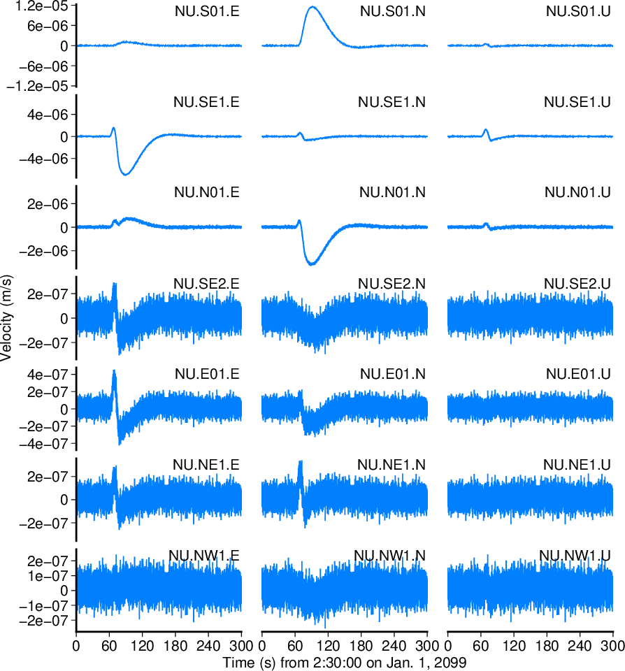
図1-2. 生波形。
Fig. 1-2. Raw waveforms.

図1-2を見ると山頂に近いNU.S01, NU.SE1, NU.N01の3観測点では 上下動において時刻60 sあたりから約20秒のパルス幅の超長周期イベントが見られる。 水平動のパルス幅が遥かに長いのは広帯域地震計の傾斜応答の影響と思われる。 残りの4観測点は山頂からやや遠く(図1-1)、振幅が小さく、シグナル/ノイズ比が小さい。
The vertical waveforms at stations NU.S01, NU.SE1, and NU.N01 in Fig. 1-2 show a very long period (VLP) event of ~ 20 s pulse width starting at ~ 60 s; these stations are located near the summit. The pulse durations in the horizontal component are substantially longer than those in the vertical one probably because of the instrumental response to tilt. The other four stations are relatively distant from the summit (Fig. 1-1) and show small amplitudes and low signal-to-noise ratios.


1-4-2. ローパスフィルター (Low-pass filtering)

図1-2では遠方の観測点で高周波ノイズに隠れて超長周期イベントが見えない。 そこでローパスフィルターを掛けてみる。 ローパスフィルターはSACソフトウェアを用いて掛けることもできるが、 ymaeda_opentoolsの sequencefile_lowpassコマンド を用いて掛けることもできる。 後者の方法で1 Hzのローパスフィルターを掛けるbashコマンドを以下に示す。
In Fig. 1-2, the VLP events are hidden by high-frequency noise at distant stations. To find the VLP events at these stations, let us try to apply a low-pass filter. The filter can be applied by SAC software, or alternatively by sequencefile_lowpass command of ymaeda_opentools. Bash commands based on the latter approach for a low-pass filter of 1 Hz are shown below.

cd waveforms
for rawfile in NU.???.?.seq2
do
     lpfile=`basename $rawfile .seq2`
     lpfile=${lpfile}.lp1Hz.seq2
     sequencefile_lowpass $rawfile $lpfile --cornerFreq=1.0
done
cd ..

これにより「観測点コード.成分コード.lp1Hz.seq2」の名前のファイルが作られる。 これらをプロットするには1-4-1節で作成したスクリプトで 入力ファイル名の「.seq2」を「.lp1Hz.seq2」に、 変数outputfile_noExtで指定する出力(画像)ファイル名を 別の名前(例えばwaveforms_lp1Hz)に変更すれば良い。 プロットしたグラフが図1-3である。
By this, files with names “station.component.lp1Hz.seq2” are created. To plot them, just modify the input file names from “.seq2’ to “.lp1Hz.seq2’ and rename the output (image) file name specified by variable outputfile_noExt to another one (e.g., waveforms_lp1Hz) in the script created in Section 1-4-1. The result is Fig. 1-3.


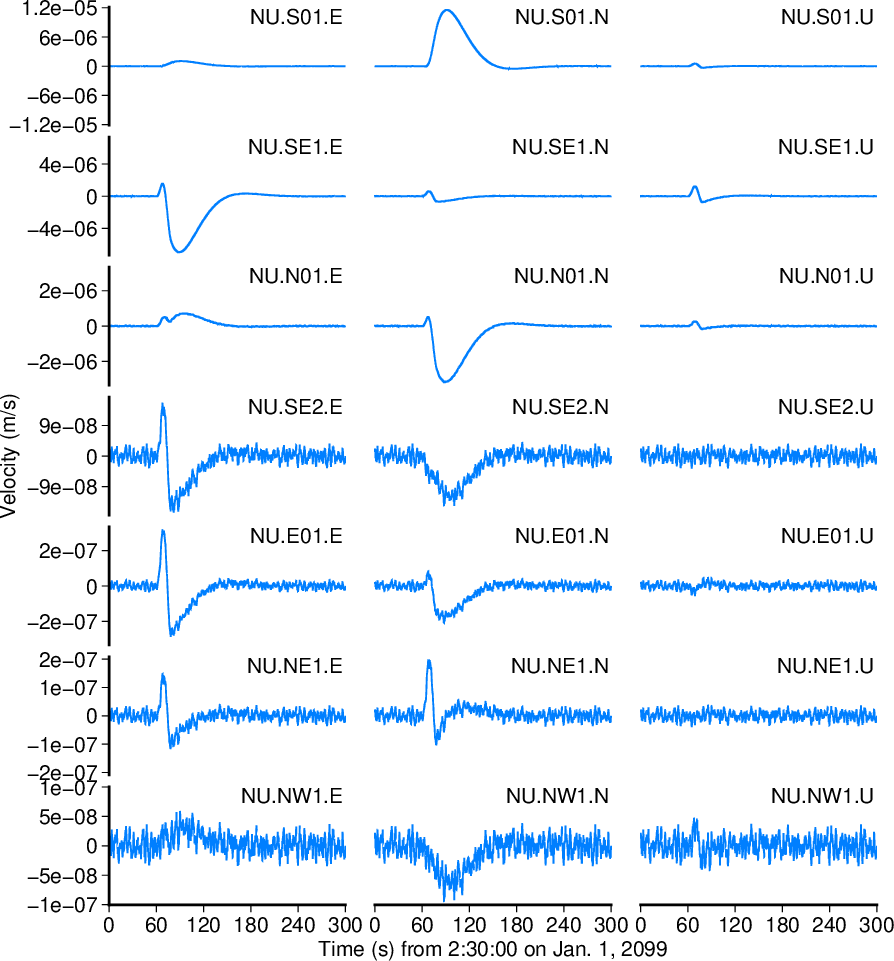
図1-3. 1 Hzのローパスフィルターを掛けた波形。
Fig. 1-3. Waveforms low-pass-filtered at 1 Hz.

ローパスフィルターにより、遠方の観測点においても超長周期イベントが見やすくなった。 しかし0.2 Hzにピークを持つ脈動ノイズが重なっている。 そこで次に0.1 Hzのローパスフィルターを掛けてみる。 やり方は上と同じであるので割愛し、結果を図1-4に示す。
The low-passed waveforms (Fig. 1-3) show clearer VLP events at distant stations than raw waveforms (Fig. 1-2). However, microtremor at 0.2 Hz contaminates the waveforms. To drop it, let us next apply a low-pass filter of 0.1 Hz. The procedure is same as above, and the result is Fig. 1-4.


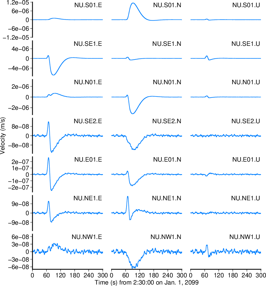
図1-4. 0.1 Hzのローパスフィルターを掛けた波形。
Fig. 1-4. Waveforms low-pass-filtered at 0.1 Hz.

図1-4を見ると図1-3よりも高いシグナル/ノイズ比が得られ、 遠方観測点においても超長周期イベントを確認できる。 0.05 Hzにピークを持つ脈動ノイズが重なっているが、 超長周期イベント自体のパルス幅が約20秒であるので これ以上の低周波のローパスフィルターを掛ければシグナル自体が損なわれると思われる。 したがって今回の解析では0.1 Hzのローパスフィルターが適切と判断できる。
The waveforms in Fig. 1-4 show a higher signal-to-noise ratios than those in Fig. 1-3, and consist of VLP events at distant stations. Although microtremor at 0.05 Hz contaminates the waveforms, a low-pass filtering with a further lower corner frequency would loose the signal because the pulse width of the VLP event is approximately 20 s. Therefeore, a low-pass filter at 0.1 Hz is considered to be a proper choise.

また図1-4を見ると5分間の波形全体を使わなくても良いことが分かる。 どの観測点・成分においても最初の30秒と最後の1分はほぼシグナルを含んでいないので、 これらを除いて2:30:30-2:34:00の波形を逆解析すれば良さそうである。
Fig. 1-4 also suggests that not the entire 5-min waveforms need to the used; the first 30 s and the last 1 min of the waveforms include almost no signal, the time window for the analysis should be 2:30:30-2:34:00.