waterPMLコマンドの検証

4. 実際の3次元地形を用いた計算

(Examples and validations for waterPML command — 4. computation using actual 3-D topography)


◆地形データの入手 (Acquiring topography data)

●概要 (Outline)

waterPMLコマンドを用いた計算の4つ目の例として、 実際の3次元地形を用いた計算を試してみる。 御嶽山周辺の地形データを使用する。
The 4th example of computation with the waterPML command uses an actual 3-D topography around Mt. Ontake, central Japan.

御嶽山に限らず日本国内の地形データは 国土地理院のWEBサイト から無償でダウンロードできる。 地形データの再配布はできないのでここではダウンロード手順を説明する。 この手順にしたがって各自でダウンロードのこと。 なお、ダウンロード手順は2024年3月5日現在のものであり、 国土地理院によって手順が変更される場合がありうる。
Topography data in Japan, not limited to Mt. Ontake, is downloadable with no charges from the WEB site of the Geospatial Information Authority of Japan (GSI). Because the data must not be redistributed, procedures to download the data are described here. Download the data by yourself following these procedures. Note that the procedures are valid as of March 5, 2024, and may be changed in the future by the GSI.


●地形データのダウンロード手順 (Procedures to download topography data)

  1. 国土地理院ホームページ の「地図情報」をクリックする。
    Click “地図情報” (map information) in the WEB site of GSI.

  2. 「基盤地図情報」をクリックする。
    Click “基盤地図情報” (basis map information).

  3. 「基盤地図情報のダウンロード」をクリックする。
    Click “基盤地図情報のダウンロード” (download basis map information).

  4. 「数値標高モデル」—「ファイル選択へ」をクリックする。
    Click “数値標高モデル” (digital elevation model) — “ファイル選択へ” (go to file selection).

  5. 1mメッシュ、5mメッシュ、10mメッシュの選択肢がある。 waterPMLコマンドによる波形計算では多くの場合、 コンピュータのメモリと計算時間の制約により 10 mよりも粗いメッシュで計算することになる。 したがって10 mメッシュで十分である。 「10mメッシュ」を選択する。
    Data of 1 m, 5 m, and 10 m meshes are available. Most computation of waveforms by waterPML command uses meshes coarser than 10 m to save memory requirements and computation time. Therefore, data of 10 m mesh is fine enough. Choose “10mメッシュ” (10 m mesh).

    なお「10mメッシュ」という名前であるが 厳密には緯度経度の0.4秒毎に標高が与えられており、 直交座標系に変換すると厳密には10 m間隔ではない。
    Despite the name “10 m mesh”, the elevation data is given at every 0.4 s in the latitude and longitude; the data is not exactly given at 10 m intervals when converted to a cartesian coordinate system.

  6. メッシュ番号の533763, 533764, 533773, 533774が御嶽山山頂周辺エリアである。 これらを地図から選択またはメッシュ番号で選択する。
    Meshes 533763, 533764, 533773, and 533774 corresponding to areas around the summit of Mt. Ontake. Choose them from the map or by mesh numbers.

    なおメッシュ番号は以下の考え方で割り出せる。
    The mesh indices were identified by the following procedure.

  7. 「ダウンロードファイル確認へ」をクリックする。
    Click “ダウンロードファイル確認へ” (confirm download files).

  8. 4つのzipファイルにチェックを入れて「まとめてダウンロード」をクリックする。
    Check the four zip files and click “まとめてダウンロード” (download all).

  9. ログインIDとパスワードでログインする。 初めての利用の場合は「新規登録」からユーザ登録を行う。
    Login by “ログインID” (login ID) and “パスワード” (password). If this is the first use, click “新規登録” (new registeration) to create a new user account.

  10. 利用目的を尋ねられる。「教育研究」にチェックを入れて 「次へ(アンケートの送信も自動で行います)」をクリックする。
    You are asked the purpose of the data download. Check “教育研究” (education and research) and click “次へ(アンケートの送信も自動で行います)” (next; automatically send your answer of the purpose).

  11. 「複数のファイルを選択した場合、ダウンロードが長時間にわたる場合があります」 のメッセージが表示されるので「OK」をクリックする。
    A message is displayed, which informs that the download of multiple files may take time. Click “OK” to proceed.

  12. 地形データが手元のコンピュータにダウンロードされる。
    The topography data is downloaded to your local computer.


◆地形データの整形 (Reformatting topography data)

ダウンロードしたファイルはPackDLMap.zipという名前である。 これを専用のディレクトリ(ここでは例としてDEMdataというディレクトリにする)に置いて解凍する。
The name of the downloaded file is PackDLMap.zip. Place it in a directory for topography (named DEMdata in the description below) and uncompress it.

mkdir DEMdata
cd DEMdata
mv ~/Download/PackDLMap.zip .
unzip PackDLMap.zip

すると以下の4つのzipファイルが作られる。
Then, the four zip files listed below are created.


これらはダウンロードのステップ6で選択した領域毎の地形データである。 ほかにxmlファイルが作られるが、それらは削除して構わない。
These are the topography data in individual regions selected in the step 6 of download procedures. In addition, xml files are created; they are not necessary and can be removed.

rm -f *.xml

次に、領域毎の地形データのzipファイルを解凍する。
Next, uncompress the topography data in individual regions.

unzip FG-GML-5337-63-DEM10B.zip
unzip FG-GML-5337-64-DEM10B.zip
unzip FG-GML-5337-73-DEM10B.zip
unzip FG-GML-5337-74-DEM10B.zip

これにより、以下の4つのファイルが作られる。
By this, the four files listed below are created.


これらのファイルには4つの地域それぞれにおける 緯度経度の0.4秒毎の標高データが格納されている。 ファイルはXML形式であるが、ymaeda_opentoolsの GSIdem2latlonDataコマンド を用いれば緯度・経度・標高の組の一覧表形式に変換できる。 以下がコマンドの例である。
These files consist of the elevation data at every 0.4 s in the latitude and longitude in the four regions. The data are written in XML format and can be converted to a table of the combination of the latitude, longitude, and elevation at each mesh node by GSIdem2latlonData command in ymaeda_opentools. An example of the command run is shown below.

GSIdem2latlonData FG-GML-5337-63-dem10b-20161001.xml 5337-63.dat
GSIdem2latlonData FG-GML-5337-64-dem10b-20161001.xml 5337-64.dat
GSIdem2latlonData FG-GML-5337-73-dem10b-20161001.xml 5337-73.dat
GSIdem2latlonData FG-GML-5337-74-dem10b-20161001.xml 5337-74.dat

これにより、5337-63.dat, 5337-64.dat, 5337-73.dat, 5337-74.dat の4つのファイルが作成される。 これらのファイルの中身は第1列が緯度、第2列が経度、第3列が標高になっており、 地図にプロットしたり特定の地点の標高を調べるのが容易である。 waterPMLコマンドではこれらのファイルを地形データとして直接用いることができる。
By this, files 5337-63.dat, 5337-64.dat, 5337-73.dat, and 5337-74.dat are created. The 1st to 3rd columns in each line of these files indicate the latitude, longitude, and elevation, respectively. Data in this format can easily be plotted in a map, and we can easily survey the elevation at a specific location from these files. The waterPML command can directly read these topography data in this format.


◆コマンド (The command)

上で作成した地形データを用いるwaterPMLコマンドの実行例を以下に示す。
An example of the waterPML command run is shown below, where the topography data created above is used.

waterPML --Nx=101 --Nz=32 --x0=-5050.0 --y0=-5050.0 --z0=0.0 --dx=100.0 --Npmx=20 --dt=0.01 --tmax=20.0 --structure_file=structure_ontake.ini --structure_file_format=layer --source_file=source_ontake.ini --output_dir=result04 --station_file=station_list4.dat --snapshot_grid=specify:file=snapshot4.ini --snapshot_dt=1.0 --topography_files=DEMdata/5337-63.dat,DEMdata/5337-64.dat,DEMdata/5337-73.dat,DEMdata/5337-74.dat --topography_file_format=latlon --refN=35:53:34 --refE=137:28:49 --output_parameters=yes

この例では上で作成した地形ファイルを --topography_files オプションで読み込んでいる。 4つのファイルがあるが、このようにカンマ(,)で区切って並べれば良い。
This example reads the topography files created above by --topography_files option, in which the four files are separated by commas (,).

waterPMLコマンドでは直交座標系を使用する。 地形データは緯度経度で与えられているので変換が必要である。 変換自体はプログラム内部で自動で行われるので、 ユーザが気にするべきポイントは以下の2点である。
The waterPML command is based on a cartesian coordinate system. The topography data, given with the latitude and longitude, has to be converted to the cartesian. This conversion is performed automatically within the program. Users must be aware of the following two points.

このように緯度経度から直交座標への基準点を指定した場合、 その地点が\((x,y)=(0,0)\)となる。 また数値標高モデルでは各地点での標高が海抜で与えられているので、 それと整合的になるように\(z\)座標の原点を海水準に設定する。 --Nx=101 --Nz=32 --x0=-5050.0 --y0=-5050.0 --z0=0.0 --dx=100.0 のオプションはこれらを踏まえたものである。 メモリと計算時間を抑えるために100 mの格子セルを用いており、 物理領域の範囲は\(-5050\leq x,y\leq 5050\), \(0\leq z\leq 3200\) (単位:m) であるので御嶽山山頂から東西南北5 km以内かつ海水準から上の範囲で計算が行われる。 御嶽山山頂の標高が3067 mであるので格子セルで近似した地表面は最高地点で\(z=3100\) mとなり、 その上に真空の格子セルを置くために\(z\)の最大値を3200 mにしている。
When the reference point for the coordinate conversion is specified, as in this example, the coordinate origin \((x,y)=(0,0)\) is assigned at the reference point. The origin of \(z\) must be at sea level to be consistent with the digital elevation model. The options --Nx=101 --Nz=32 --x0=-5050.0 --y0=-5050.0 --z0=0.0 --dx=100.0 are based on this coordinate system. A grid cell size of 100 m is used to save computation memory and time, and the physical volume extends over \(-5050\leq x,y\leq 5050\), \(0\leq z\leq 3200\) (unit: m), which means that the computation is performed in a 10 km × 10 km region centered on the summit of Mt. Ontake and above sea level. The maximum value of \(z\) is chosen as 3200 m because the summit elevation of Mt. Ontake is 3067 m, which is approximated by 3100 m in the grid cell system; at least one vacuum cell is needed to express a ground surface.

Maeda et al. (2011)ではPML領域に10格子セルを用いたが、 それ以降の計算では人為的な境界からの反射波をより確実に抑えるために 20格子セルを用いており、今回の計算でもそれを踏襲している(--Npmx=20)。
Maeda et al. (2011) used 10 grid cells in the PML volume; however, later computations used 20 grid cells to better suppress the waves reflected from artificial boundaries. The example above follows this treatment (--Npmx=20).

経験上、時間刻み(s)は格子セルサイズ(m)の1/10000以下にする必要があるので 0.01 s刻みとした(--dt=0.01)。
My experiences indicate that a time stepping (s) must be less than or equal to 1/10000 times a grid cell size (m); therefore, a time stepping of 0.01 s is used (--dt=0.01).

今回の例では--output_parameters=yesオプションを用いた。 これにより、例えば地形データが格子セルによってどのように近似されたか等、 格子セルレベルでの計算条件の詳細を出力できる。
This example uses --output_parameters=yes option to show computation conditions as fine as grid cell level; for example, how the topography is approximated by grid cells.

地下構造、地震波動ソース、観測点、スナップショットの設定は下記の通りである。
Configurations for the subsurface structure, seismic wave source, stations, and snapshots are described below.


●地下構造 (Subsurface structure)

御嶽山における地下構造の推定結果(Maeda and Watanabe 2023)に基づき P波速度\(V_p\)を以下のように与える。
P-wave velocities \(V_p\) are given as below, based on a structural survey in Mt. Ontake by Maeda and Watanabe (2023).


Layer
標高
Elevation (above sea level)
P波速度(m/s)
P-wave velocity
新期御嶽
Younger Ontake
> 1900 m 2400 m/s
古期御嶽
Older Ontake
900-1900 m 3600 m/s
基盤岩
Basement
< 900 m 5600 m/s

S波速度は\(V_s=V_p/\sqrt{3}\)とし、 密度はGardner (1974)に基づいて \(\rho\) (kg/m\(^3\)) \(=1700+0.2V_p\) (m/s)とした。
S-wave velocities are calculated as \(V_s=V_p/\sqrt{3}\), and densities are calculated as \(\rho\) (kg/m\(^3\)) \(=1700+0.2V_p\) (m/s) based on Gardner (1974).

この地下構造は以下のファイルで表現できる。 物理領域の\(z\)座標の範囲をカバーするように \(-100\leq z\leq 3300\)の範囲の地下構造を与えている。 なお地下構造の設定ファイルで表現できるのは\(z\)の区分線形関数であるので、 層境界には僅かに厚みを持たせてその範囲で\(z\)の1次関数として物性値を変化させている。
This subsurface structure is expressed by the file below, which extends over \(-100\leq z\leq 3300\) to bound the \(z\)-coordinate range of the physical volume. Note than a slight but finite thickness is given to layer boundaries because the file assumes piecewise linear functions of \(z\).

(structure_ontake.ini)
3300.0[TAB]2400.0[TAB]1385.6[TAB]2180.0
1900.1[TAB]2400.0[TAB]1385.6[TAB]2180.0
1899.9[TAB]3600.0[TAB]2078.5[TAB]2420.0
900.1[TAB]3600.0[TAB]2078.5[TAB]2420.0
899.9[TAB]5600.0[TAB]3233.2[TAB]2820.0
-100.0[TAB]5600.0[TAB]3233.2[TAB]2820.0

このファイルは --structure_file=structure_ontake.ini --structure_file_format=layer オプションによって計算に取り込まれる。
The subsurface structure given in this file is incorporated into the computation by --structure_file=structure_ontake.ini --structure_file_format=layer options.


●地震波動ソース (Seismic wave source)

今回の例題では地震波動ソースとして 2014年噴火直前の超長周期地震(Maeda et al. 2015)のソース位置 (山頂から西に360 m、南に480 m、標高2040 m) とメカニズム (走向354°、傾斜角79°の開口クラック) を用いる。 震源時間関数はMaeda et al. (2015)で バンドパスフィルターの影響を除去した震源時間関数 (deconvolved form of the source time function; DSTF) として求めた最大振幅\(5.2\times 10^{11}\) N m、時定数7 sのガウス関数とする。 この地震波動ソースは以下のファイルで与えられる。
This example uses the location (360 m west and 480 m south from the summit, 2040 m above sea level) and mechanism (a tensile crack striking 354° and dipping 79°) of the source of the very long period event that immediately preceded the 2014 eruption (Maeda et al. 2015) as the seismic wave source. The deconvolved form of the source time function (DSTF) estimated by Maeda et al. (2015) is used as the source time function, which is a Gaussian function of 7 s duration with a maximum amplitude of \(5.2\times 10^{11}\) N m. This seismic wave source is given by the file below.

(source_ontake.ini)
newsource VLP2014
location_x=-360.0
location_y=-480.0
location_z=2040.0
mechanism=point_tensile
intensity=5.2e+11
theta=79.0
phi=6.0
stfun_name=gaussian
stfun_tp=7.0
stfun_ts=3.5

このファイルは --source_file=source_ontake.ini オプションによって計算に取り込まれる。 また経験上、時定数7 sの震源時間関数であれば 20 s間の波形を計算すれば最終時刻までに振幅がほぼ0に収まるので 計算時間を20 sとした(--tmax=20.0)。
The configuration of this source is incorporated into the computation by --source_file=source_ontake.ini option. My experiences indicate that the amplitude of the wave would converge to almost zero before 20 s in case of a source time function of 7 s duration; therefore, a time length of 20 s is used (--tmax=20.0).


●観測点 (Stations)

観測点の座標は通常、緯度経度で与えられるので直交座標系に変換する必要がある。 この変換にはymaeda_opentoolsの latlon2xyコマンド が利用できるが、その際の基準点はwaterPMLコマンドと同じ場所 (今回の例であれば北緯35度53分34秒、東経137度28分49秒) を使わなければならない。
Station coordinates are usually given in latitudes and longitudes, which must be converted to cartesian coordinates. The latlon2xy command in ymaeda_opentools is available for this conversion. The reference point of the conversion must be same as that of the waterPML command (35°53’34”N, 137°28’49”E in this example).

実際の観測点の情報はこのサイトでの公開には適さないため 今回の例題では以下の2つの仮想的な観測点を使用する。 1つ目の観測点をNU.ONTK1とし、 北緯35.884度、東経137.525度の位置で地表置きとする。 2つ目の観測点をNU.ONTK2とし、 北緯35.865度、東経137.496度の位置で深さ150 mのボアホールとする。 これらの観測点の直交座標を求めるコマンドを以下に示す。
Information for actual stations should not be opened in this site; therefore, this example uses the following two virtual stations. One is a station NU.ONTK1 located at the ground surface of 35.884°N, 137.525°E. The other is a station NU.ONTK2 located at the bottom of a 150 m borehole beneath 35.865°N, 137.496°E. Commands to compute the cartesian coordinates of these stations are shown below.

latlon2xy --N=35.884 --E=137.525 --refN=35:53:34 --refE=137:28:49
latlon2xy --N=35.865 --E=137.496 --refN=35:53:34 --refE=137:28:49

refN, refEの値をwaterPMLコマンドと同じにしている点が重要である。 コマンドを実行すると\(x\)座標(東、m)、\(y\)座標(北、m)の順に 計算結果が画面に表示される。 NU.ONTK1は\(x=4037.8138\) m, \(y=-972.9342\) m、 NU.ONTK2は\(x=1419.8436\) m, \(y=-3081.7098\) mと計算される。 これらの値に基づき、下記の観測点リストファイルを作成する。
Note that the values of refN and refE are same as those in the waterPML command. The latlon2xy command displays an \(x\)-coordinate (east, m) followed by a \(y\)-coordinate (north, m); the results are \(x=4037.8138\) m and \(y=-972.9342\) m for NU.ONTK1 and \(x=1419.8436\) m and \(y=-3081.7098\) m for NU.ONTK2. Using these values, create a station list file as below.

(station_list4.dat)
NU.ONTK1[TAB]4037.8138[TAB]-972.9342[TAB]surface-0.1
NU.ONTK1.W1[TAB]3937.8138[TAB]-972.9342[TAB]surface-0.1
NU.ONTK1.W2[TAB]3837.8138[TAB]-972.9342[TAB]surface-0.1
NU.ONTK1.E1[TAB]4137.8138[TAB]-972.9342[TAB]surface-0.1
NU.ONTK1.E2[TAB]4237.8138[TAB]-972.9342[TAB]surface-0.1
NU.ONTK1.S1[TAB]4037.8138[TAB]-1072.9342[TAB]surface-0.1
NU.ONTK1.S2[TAB]4037.8138[TAB]-1172.9342[TAB]surface-0.1
NU.ONTK1.N1[TAB]4037.8138[TAB]-872.9342[TAB]surface-0.1
NU.ONTK1.N2[TAB]4037.8138[TAB]-772.9342[TAB]surface-0.1
NU.ONTK2[TAB]1419.8436[TAB]-3081.7098[TAB]surface-150.0
NU.ONTK2.W1[TAB]1319.8436[TAB]-3081.7098[TAB]surface-150.0
NU.ONTK2.W2[TAB]1219.8436[TAB]-3081.7098[TAB]surface-150.0
NU.ONTK2.E1[TAB]1519.8436[TAB]-3081.7098[TAB]surface-150.0
NU.ONTK2.E2[TAB]1619.8436[TAB]-3081.7098[TAB]surface-150.0
NU.ONTK2.S1[TAB]1419.8436[TAB]-3181.7098[TAB]surface-150.0
NU.ONTK2.S2[TAB]1419.8436[TAB]-3281.7098[TAB]surface-150.0
NU.ONTK2.N1[TAB]1419.8436[TAB]-2981.7098[TAB]surface-150.0
NU.ONTK2.N2[TAB]1419.8436[TAB]-2881.7098[TAB]surface-150.0

ここでは各観測点から東西南北2つ目までの格子セルにも観測点を置いた。 例えばNU.ONTK1.W1はNU.ONTK1の1つ西の格子セル、 NU.ONTK1.S2はNU.ONTK1の2つ南の格子セルである。 Maeda et al. (2011)では隣接する5つの格子セルでの傾斜変動を平均することを推奨している。 そのためにはこの例のように観測点に隣接する格子セルにも観測点を置いておく必要がある。
Here, stations are added to next or 2nd next grid cells of each station in east, west, south, and north directions. For example, NU.ONTK1.W1 is located at by 1 grid west of NU.ONTK1, and NU.ONTK1.S2 is located at by 2 grids south of NU.ONTK1. Maeda et al. (2011) recommends to average the tilt at five adjacent grid cells. To do it, stations have to be placed at the next or 2nd next grid cells.

観測点の標高(第4列)はGPSで計測した標高ではなく、 上の例のように地表からの深さで指定すべきである。 GPSで計測した標高を用いた場合、 GPSや数値標高モデルの僅かな誤差によって観測点が空中に置かれてしまう恐れがある。 surface-0.1のように地表からの深さで指定すれば 数値標高モデルに基づいて設定した地表面よりも下に確実に観測点を置いて計算が行われる。
The station elevations (4th column) should not be given as the values measured by GPS but should be given as the depth from the ground surface, as the example above shows. If a measured station elevation is used, it may be in the vacuum region above the ground surface, depending on small errors in the GPS measurement and digital elevation model. If a station elevation is specified as the depth from the ground surface, for example as surface-0.1, the station is guaranteed to be located beneath the ground surface from the digital elevation model in the computation.

ファイルstation_list4.datは --station_file=station_list4.dat オプションによって計算に取り込まれる。
The file station_list4.dat is incorporated into the computation by --station_file=station_list4.dat option.


●スナップショット (Snapshots)

今回の例題では御嶽山山頂を通る東西断面(\(y=0\))でのスナップショットを出力してみる。
Let us output the snapshots along an EW transect that passes through the summit of Mt. Ontake (\(y=0\)).

(snapshot4.ini)
newsnap EWsection_y0
snapname EWsection_y0
xrange -5000.0,5000.0
yrange -1.0,1.0
zrange 0.0,3200.0

このファイルは --snapshot_grid=specify:file=snapshot4.ini オプションによって計算に取り込まれる。
The configuration in this file is incorporated into the computation by --snapshot_grid=specify:file=snapshot4.ini option.


◆スナップショットの確認 (Checking the snapshots)

ここでは例として時刻\(t=3\) sでの速度場の\(x\)成分のスナップショットをプロットしてみる。 例題1 と考え方は同様であるのでプロット用のコマンドのみを以下に示す。
Let us plot the snapshot for the \(x\)-component velocity field at time \(t=3\) s as an example. This work is similar to that described in the 1st example; therefore, only the commands to plot the snapshot are shown below.

cd result04/snapshot

3d_data_convert EWsection_y0.Vx.t3.0000 3db 3d

gmt begin EWsection_y0.Vx.t3.0000 ps

gmt set FONT_ANNOT_PRIMARY 12p

awk 'BEGIN{ FS="\t" }(NF==4){ print $1,$3,$4*1e+6 }' EWsection_y0.Vx.t3.0000.3d | gmt xyz2grd -R-5000/5000/50/3150 -I100/100 -GEWsection_y0.Vx.t3.0000.grd

gmt makecpt -Cpolar -T-8/8/0.1 -Z -D

gmt grdimage EWsection_y0.Vx.t3.0000.grd -R-5000/5000/0/3200 -JX10/3.2 -Xa3 -Ya5 -Bxa2000f1000 -By1000f500 -BWSen

gmt colorbar -Dx8/3/6/0.5h -Bxa4f1 -BS

gmt text -R0/21/0/29.7 -JX21/29.7 -Xa0 -Ya0 -F+f12p+a+j <<EOF
8 4.2 0 CT East (m) from the summit
1.5 6.6 90 CB Elevation (m)
8 1.7 0 CT Velocity Vx (10@+-6@+ m/s)
EOF

gmt end

cd ../..

これによりresult04/snapshotディレクトリの下に EWsection_y0.Vx.t3.0000.psのファイル名でスナップショットがプロットされる。 この画像を図1に示す。 地表面よりも上(真空の格子セル)では振幅が0になるのでこの図では白になり、 色付きの領域が山体の形を表している。 ソースのクラックを挟んで東側や上側が東方向(赤色)、西側や下側が西方向(青色)の動きを示しており、 与えた開口クラックソースから期待される動きと整合的である。 一方で短波長の振幅変化が見られ、 今回の格子セルサイズ(100 m)では波動場を十分に表現できていない可能性がある。 なおMaeda et al. (2015)では40 mの格子セルを使用した。
By this, a snapshot is plotted in a file EWsection_y0.Vx.t3.0000.ps (shown in Fig. 1.) under a directory result04/snapshot. Above the ground surface (in vacuum cells) the amplitude is zero and thus plotted by white color. As a result, the colored region represents the topography of the mountain. The material moves eastward (red color) in eastern and upper regions and westward (blue color) in western and lower regions of the tensile crack soruce, consistent with an expected pattern of the motion. However, short-wavelength spatial variation of amplitudes may not be satisfactory expressed by the 100 m grid cells used in this example. Maeda et al. (2015) used 40 m grid cells.


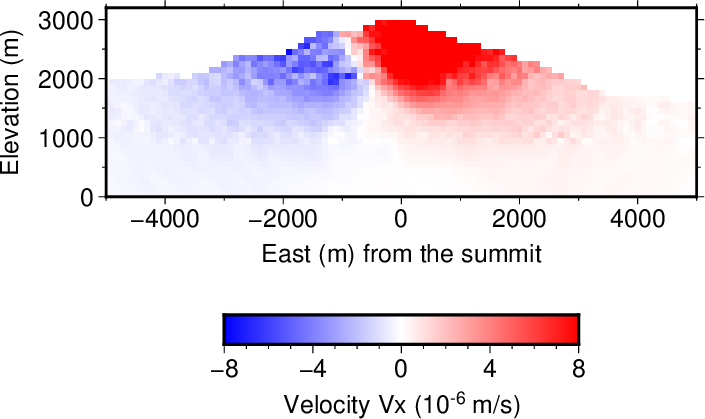
図1. 時刻\(t=3\) sでの速度の\(x\)成分\(V_x\)のスナップショット (山頂を通る東西断面)。
A snapshot of the \(x\)-component velocity \(V_x\) at time \(t=3\) s along an EW transect that passes through the summit.


◆速度波形の確認 (Checking the velocity waveforms)

2つの観測点での速度波形3成分をプロットしてみる。 これまでの例題では解析解との比較のために速度波形を積分して変位波形に直したが、 今回は速度波形のままで良い。 前処理として必要な作業はseq1形式からseq2形式への変換のみであり、 ymaeda_opentoolsの sequencefile_convertコマンド を用いて変換できる。
Let us plot the 3-component velocity waveforms at the two stations. Previous examples integrated the velocity waveforms to displacement for comparison with analytical solutions. In this example, the integration is not needed. Only a conversion of file format from seq1 to seq2 is needed, for which sequencefile_convert command in ymaeda_opentools is available.

cd result04/waveform
for station in NU.ONTK1 NU.ONTK2
do
  for component in Vx Vy Vz
  do
    sequencefile_convert $station.$component seq1 seq2
  done
done

変換後はこれまでと同様、 Generic Mapping Tools (version 6) を用いてプロットする。
After the conversion, plot the data by Generic Mapping Tools (version 6), as in the previous examples.

gmt begin velocity ps

gmt set FONT_ANNOT_PRIMARY 12p

awk '(NF==2){ print $1,$2*1e+06 }' NU.ONTK1.Vx.seq2 | gmt plot -R0/20/-3/3 -JX6/2 -Xa3 -Ya7 -W1,0/127/255 -Bxa5f1 -Bya2f1 -BWsen

awk '(NF==2){ print $1,$2*1e+06 }' NU.ONTK1.Vy.seq2 | gmt plot -R0/20/-3/3 -JX6/2 -Xa3 -Ya5 -W1,0/127/255 -Bxa5f1 -Bya2f1 -BWsen

awk '(NF==2){ print $1,$2*1e+06 }' NU.ONTK1.Vz.seq2 | gmt plot -R0/20/-3/3 -JX6/2 -Xa3 -Ya3 -W1,0/127/255 -Bxa5f1 -Bya2f1 -BWSen

awk '(NF==2){ print $1,$2*1e+06 }' NU.ONTK2.Vx.seq2 | gmt plot -R0/20/-3/3 -JX6/2 -Xa10 -Ya7 -W1,0/127/255 -Bxa5f1 -Bya2f1 -Bwsen

awk '(NF==2){ print $1,$2*1e+06 }' NU.ONTK2.Vy.seq2 | gmt plot -R0/20/-3/3 -JX6/2 -Xa10 -Ya5 -W1,0/127/255 -Bxa5f1 -Bya2f1 -Bwsen

awk '(NF==2){ print $1,$2*1e+06 }' NU.ONTK2.Vz.seq2 | gmt plot -R0/20/-3/3 -JX6/2 -Xa10 -Ya3 -W1,0/127/255 -Bxa5f1 -Bya2f1 -BwSen

gmt text -R0/21/0/29.7 -JX21/29.7 -Xa0 -Ya0 -F+f12p+a+j <<EOF
6 2.3 0 CT Time (s)
13 2.3 0 CT Time (s)
2 6 90 CB Velocity (10@+-6@+ m/s)
8.8 8.8 0 RT NU.ONTK1 (EW)
8.8 6.8 0 RT NU.ONTK1 (NS)
8.8 4.8 0 RT NU.ONTK1 (UD)
15.8 8.8 0 RT NU.ONTK2 (EW)
15.8 6.8 0 RT NU.ONTK2 (NS)
15.8 4.8 0 RT NU.ONTK2 (UD)
EOF

gmt end

これにより、result04/waveformディレクトリの下に velocity.psのファイル名で波形がプロットされる。 この画像を図2に示す。 おおよそ3 s程度の周期の振動成分が見られ、特に東西成分で明瞭である。 最も遅い新期御嶽のS波速度で考えても周期3 sはおおよそ波長4 kmに対応し、 1波長に40格子セルが入ることから、 この周期の振動成分については計算結果に信頼性があると考えられる。
By this, the waveforms are plotted in a file velocity.ps (shown in Fig. 2) under a directory result04/waveform. They consistent of oscillations in ~ 3 s period, which are clear especially in the EW component. The period of 3 s corresponds to a wavelength of 4 km in case of the slowest S-wave velocity in the younger Ontake. This wavelength includes 40 grid cells, suggesting that the computation results in this period are reliable.


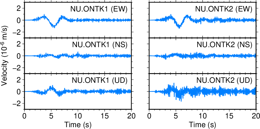
図2. 2つの仮想観測点での速度波形。
Fig. 2. Velocity waveforms at the two virtual stations.

一方、図2には短周期の振動成分も記録されており、これらには信頼性が無いと思われる。 ymaeda_opentoolsの sequencefile_lowpassコマンド を用いると時系列データにローパスフィルターを掛けることができる。 このコマンドを使用し、速度波形に1 Hzのローパスフィルターを掛ける例を以下に示す。
Fig. 2 also records short-period oscillations, which are considered unreliable. Therefore, apply a low-pass filter of 1 Hz to these time series data using sequencefile_lowpass command as shown below.

for station in NU.ONTK1 NU.ONTK2
do
  for component in Vx Vy Vz
  do
    sequencefile_lowpass $station.$component.seq2 $station.$component.lp1Hz.seq2 --cornerFreq=1.0
  done
done

これにより「観測点名.成分名.lp1Hz.seq2」(例:NU.ONTK1.Vx.lp1Hz.seq2)の名前で ローパスフィルターを掛けた波形データが出力される。 これらを生波形のときと同じ要領でプロットする。
By this, the low-passed waveforms are written into files with names “station code.component code.lp1Hz.seq2” (e.g., NU.ONTK1.Vx.lp1Hz.seq2). Plot them in the same manner as raw waveforms.

gmt begin velocity_lp1Hz ps

gmt set FONT_ANNOT_PRIMARY 12p

awk '(NF==2){ print $1,$2*1e+06 }' NU.ONTK1.Vx.lp1Hz.seq2 | gmt plot -R0/20/-3/3 -JX6/2 -Xa3 -Ya7 -W1,0/127/255 -Bxa5f1 -Bya2f1 -BWsen

awk '(NF==2){ print $1,$2*1e+06 }' NU.ONTK1.Vy.lp1Hz.seq2 | gmt plot -R0/20/-3/3 -JX6/2 -Xa3 -Ya5 -W1,0/127/255 -Bxa5f1 -Bya2f1 -BWsen

awk '(NF==2){ print $1,$2*1e+06 }' NU.ONTK1.Vz.lp1Hz.seq2 | gmt plot -R0/20/-3/3 -JX6/2 -Xa3 -Ya3 -W1,0/127/255 -Bxa5f1 -Bya2f1 -BWSen

awk '(NF==2){ print $1,$2*1e+06 }' NU.ONTK2.Vx.lp1Hz.seq2 | gmt plot -R0/20/-3/3 -JX6/2 -Xa10 -Ya7 -W1,0/127/255 -Bxa5f1 -Bya2f1 -Bwsen

awk '(NF==2){ print $1,$2*1e+06 }' NU.ONTK2.Vy.lp1Hz.seq2 | gmt plot -R0/20/-3/3 -JX6/2 -Xa10 -Ya5 -W1,0/127/255 -Bxa5f1 -Bya2f1 -Bwsen

awk '(NF==2){ print $1,$2*1e+06 }' NU.ONTK2.Vz.lp1Hz.seq2 | gmt plot -R0/20/-3/3 -JX6/2 -Xa10 -Ya3 -W1,0/127/255 -Bxa5f1 -Bya2f1 -BwSen

gmt text -R0/21/0/29.7 -JX21/29.7 -Xa0 -Ya0 -F+f12p+a+j <<EOF
6 2.3 0 CT Time (s)
13 2.3 0 CT Time (s)
2 6 90 CB Velocity (10@+-6@+ m/s)
8.8 8.8 0 RT NU.ONTK1 (EW)
8.8 6.8 0 RT NU.ONTK1 (NS)
8.8 4.8 0 RT NU.ONTK1 (UD)
15.8 8.8 0 RT NU.ONTK2 (EW)
15.8 6.8 0 RT NU.ONTK2 (NS)
15.8 4.8 0 RT NU.ONTK2 (UD)
EOF

gmt end

作成された画像(velocity_lp1Hz.ps)を図3に示す。 短周期成分が抑制され、長周期の振動成分が明瞭になった。
The result is velocity_lp1Hz.ps (Fig. 3), showing clearer long-period oscillations than Fig. 2 owing to reduced short-period oscillations.


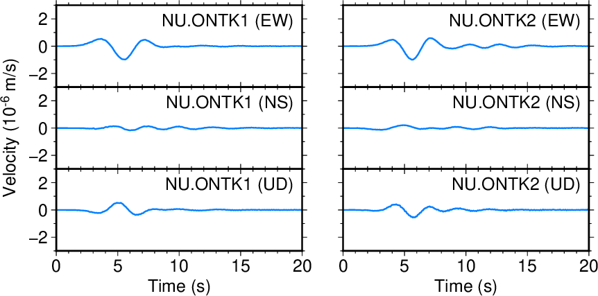
図3. 2つの仮想観測点での速度波形(ローパス1Hz)。
Fig. 3. Low-passed (1 Hz) velocity waveforms at the two virtual stations.


◆傾斜変動の波形の確認 (Checking the tilt waveforms)

傾斜変動レートの波形も速度波形と同様、 result04/waveformディレクトリの下に格納されている。 「.Tx.seq1」「.Ty.seq1」で終わる名前のファイルが傾斜変動レートの波形である。 これらは速度の上下成分\(V_z\)の水平方向への空間微分 \(\PartialDiff{V_z}{x}\), \(\PartialDiff{V_z}{y}\) になっている。
Tilt-rate waveforms are stored under the directory result04/waveform, same as velocity waveforms. Files with names that end with “.Tx.seq1’ and “.Ty.seq1’ are the data for tilt-rate waveforms. They are defined as the spatial derivatives of vertical velocity \(V_z\) along horizontal directions (\(\PartialDiff{V_z}{x}\) and \(\PartialDiff{V_z}{y}\)).

ボアホールの観測点(NU.ONTK2)においては 速度の水平成分\(V_x\), \(V_y\)の上下方向への空間微分 \(-\PartialDiff{V_x}{z}\), \(-\PartialDiff{V_y}{z}\) により傾斜変動を計算することもできる。 この定義に基づく傾斜変動レートは 「.TTx.seq1」「.TTy.seq1」で終わる名前のファイルに格納されている。
At borehole stations, the tilt can also be defined as the spatial derivatives of horizontal velocities \(V_x\) and \(V_y\) along the vertical direction (\(-\PartialDiff{V_x}{z}\) and \(-\PartialDiff{V_y}{z}\)). Tilt-rates based on this definition are stored in files with names that end with “.TTx.seq1’ and “.TTy.seq1’.

Maeda et al. (2011)では隣接する5つの格子セルでの傾斜変動を 平均して用いることを推奨している。 以下では傾斜変動の\(x\)成分は\(x\)方向に隣接するセル、 \(y\)成分は\(y\)方向に隣接するセルについて平均する。 平均の計算にはymaeda_opentoolsの sequencefiles_averageコマンドを用いる。
Maeda et al. (2011) recommends to average the tilt at five adjacent grid cells. Below, \(x\)- and \(y\)-component tilts are averaged over the adjacent cells along the \(x\)- and \(y\)-directions, respectively. The sequencefiles_average command is used for computing the averages.

sequencefiles_average --inputfiles=NU.ONTK1.W2.Tx.seq1,NU.ONTK1.W1.Tx.seq1,NU.ONTK1.Tx.seq1,NU.ONTK1.E1.Tx.seq1,NU.ONTK1.E2.Tx.seq1 --outputfile=NU.ONTK1.Tx.ave5.seq1

sequencefiles_average --inputfiles=NU.ONTK1.S2.Ty.seq1,NU.ONTK1.S1.Ty.seq1,NU.ONTK1.Ty.seq1,NU.ONTK1.N1.Ty.seq1,NU.ONTK1.N2.Ty.seq1 --outputfile=NU.ONTK1.Ty.ave5.seq1

sequencefiles_average --inputfiles=NU.ONTK2.W2.Tx.seq1,NU.ONTK2.W1.Tx.seq1,NU.ONTK2.Tx.seq1,NU.ONTK2.E1.Tx.seq1,NU.ONTK2.E2.Tx.seq1 --outputfile=NU.ONTK2.Tx.ave5.seq1

sequencefiles_average --inputfiles=NU.ONTK2.S2.Ty.seq1,NU.ONTK2.S1.Ty.seq1,NU.ONTK2.Ty.seq1,NU.ONTK2.N1.Ty.seq1,NU.ONTK2.N2.Ty.seq1 --outputfile=NU.ONTK2.Ty.ave5.seq1

sequencefiles_average --inputfiles=NU.ONTK2.W2.TTx.seq1,NU.ONTK2.W1.TTx.seq1,NU.ONTK2.TTx.seq1,NU.ONTK2.E1.TTx.seq1,NU.ONTK2.E2.TTx.seq1 --outputfile=NU.ONTK2.TTx.ave5.seq1

sequencefiles_average --inputfiles=NU.ONTK2.S2.TTy.seq1,NU.ONTK2.S1.TTy.seq1,NU.ONTK2.TTy.seq1,NU.ONTK2.N1.TTy.seq1,NU.ONTK2.N2.TTy.seq1 --outputfile=NU.ONTK2.TTy.ave5.seq1

次に、これらは傾斜変動レートの波形であるので積分して傾斜変動の波形にする。
Next, integrate these tilt-rate waveforms to obtain tilt waveforms.

sequencefile_integral NU.ONTK1.Tx.ave5.seq1 NU.ONTK1.Tx.ave5.int.seq2

sequencefile_integral NU.ONTK1.Ty.ave5.seq1 NU.ONTK1.Ty.ave5.int.seq2

sequencefile_integral NU.ONTK2.Tx.ave5.seq1 NU.ONTK2.Tx.ave5.int.seq2

sequencefile_integral NU.ONTK2.Ty.ave5.seq1 NU.ONTK2.Ty.ave5.int.seq2

sequencefile_integral NU.ONTK2.TTx.ave5.seq1 NU.ONTK2.TTx.ave5.int.seq2

sequencefile_integral NU.ONTK2.TTy.ave5.seq1 NU.ONTK2.TTy.ave5.int.seq2

速度波形のときと同様、1 Hzのローパスフィルターを掛けて短周期振動を抑える。
Suppress short-period oscillations by a low-pass filter of 1 Hz, same as the velocity waveforms.

sequencefile_lowpass NU.ONTK1.Tx.ave5.int.seq2 NU.ONTK1.Tx.ave5.int.lp1Hz.seq2 --cornerFreq=1.0

sequencefile_lowpass NU.ONTK1.Ty.ave5.int.seq2 NU.ONTK1.Ty.ave5.int.lp1Hz.seq2 --cornerFreq=1.0

sequencefile_lowpass NU.ONTK2.Tx.ave5.int.seq2 NU.ONTK2.Tx.ave5.int.lp1Hz.seq2 --cornerFreq=1.0

sequencefile_lowpass NU.ONTK2.Ty.ave5.int.seq2 NU.ONTK2.Ty.ave5.int.lp1Hz.seq2 --cornerFreq=1.0

sequencefile_lowpass NU.ONTK2.TTx.ave5.int.seq2 NU.ONTK2.TTx.ave5.int.lp1Hz.seq2 --cornerFreq=1.0

sequencefile_lowpass NU.ONTK2.TTy.ave5.int.seq2 NU.ONTK2.TTy.ave5.int.lp1Hz.seq2 --cornerFreq=1.0

最後にこれらをプロットする。
Finally, plot them.

gmt begin tilt_lp1Hz ps

gmt set FONT_ANNOT_PRIMARY 12p

awk '(NF==2){ print $1,$2*1e+10 }' NU.ONTK1.Tx.ave5.int.lp1Hz.seq2 | gmt plot -R0/20/-3.8/3.8 -JX6/2 -Xa3 -Ya5 -W1,0/127/255 -Bxa5f1 -Bya2f1 -BWsen

awk '(NF==2){ print $1,$2*1e+10 }' NU.ONTK1.Ty.ave5.int.lp1Hz.seq2 | gmt plot -R0/20/-3.8/3.8 -JX6/2 -Xa3 -Ya3 -W1,0/127/255 -Bxa5f1 -Bya2f1 -BWSen

awk '(NF==2){ print $1,$2*1e+10 }' NU.ONTK2.Tx.ave5.int.lp1Hz.seq2 | gmt plot -R0/20/-3.8/3.8 -JX6/2 -Xa10 -Ya5 -W1,0/127/255

awk '(NF==2){ print $1,$2*1e+10 }' NU.ONTK2.Ty.ave5.int.lp1Hz.seq2 | gmt plot -R0/20/-3.8/3.8 -JX6/2 -Xa10 -Ya3 -W1,0/127/255

awk '(NF==2){ print $1,$2*1e+10 }' NU.ONTK2.TTx.ave5.int.lp1Hz.seq2 | gmt plot -R0/20/-3.8/3.8 -JX6/2 -Xa10 -Ya5 -W1,255/127/0 -Bxa5f1 -Bya2f1 -Bwsen

awk '(NF==2){ print $1,$2*1e+10 }' NU.ONTK2.TTy.ave5.int.lp1Hz.seq2 | gmt plot -R0/20/-3.8/3.8 -JX6/2 -Xa10 -Ya3 -W1,255/127/0 -Bxa5f1 -Bya2f1 -BwSen

gmt text -R0/21/0/29.7 -JX21/29.7 -Xa0 -Ya0 -F+f12p+a+j <<EOF
6 2.3 0 CT Time (s)
13 2.3 0 CT Time (s)
2 5 90 CB Tilt (10@+-10@+ rad)
8.8 6.8 0 RT NU.ONTK1 (EW)
8.8 4.8 0 RT NU.ONTK1 (NS)
15.8 6.8 0 RT NU.ONTK2 (EW)
15.8 4.8 0 RT NU.ONTK2 (NS)
EOF

gmt end

作成された画像(tilt_lp1Hz.ps)を図4に示す。 今回の例題では震源時間関数の時定数が比較的短いこと、観測点がやや遠方に位置していることから 傾斜変動は小さな振幅となった。 また、2種類の方法で定義した傾斜変動にはやや差異が見られる。
Fig. 4 shows the image thus created (tilt_lp1Hz.ps). A source time function with a relatively short duration and relatively distant station locations resulted in small amplitudes in the tilt. The two definitions of the tilt showed some differences.


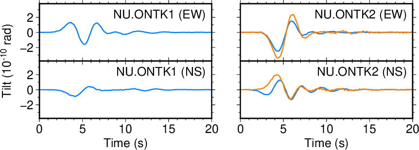
図4. 2つの仮想観測点での傾斜変動の波形(ローパス1Hz)。 青:鉛直速度の水平微分(\(\PartialDiff{V_z}{x}\), \(\PartialDiff{V_z}{y}\)) に基づく傾斜変動。 橙:水平速度の鉛直微分(\(-\PartialDiff{V_x}{z}\), \(-\PartialDiff{V_y}{z}\)) に基づく傾斜変動。
Fig. 4. Low-passed (1 Hz) tilt waveforms at the two virtual stations. Blue and orange lines show the tilts defined based on the horizontal derivatives of vertical velocity (\(\PartialDiff{V_z}{x}\), \(\PartialDiff{V_z}{y}\)) and the vertical derivatives of horizontal velocities (\(-\PartialDiff{V_x}{z}\), \(-\PartialDiff{V_y}{z}\)), respectively.


◆パラメータログの確認 (Checking parameter logs)

今回の計算では--output_parameters=yesオプションを付けたので result04ディレクトリの下にparametersサブディレクトリが作成された。 このサブディレクトリには計算条件が格子セルレベルの詳細まで記録されている。 以下、これらの情報のいくつかを紹介する。
The computation in this example used --output_parameters=yes option. Therefore, a sub directory parameters, which recorded information on computation condition as detail as grid cell level, was created under result04 directory. Some of these information are explained below.


●地震波動ソース (Seismic wave source)

result04/parameters/source.1.logはテキストファイルになっており、 その中身は以下のようになっている。
The content of a text file result04/parameters/source.1.log is as below.

name=VLP2014
location[0](specified)=-3.600000e+02
location[1](specified)=-4.800000e+02
location[2](specified)=2.040000e+03
ig(used)=5476731
n[0](used)=93
n[1](used)=91
n[2](used)=41
location[0](used)=-4.000000e+02
location[1](used)=-5.000000e+02
location[2](used)=2.050000e+03
mechanism=point_tensile
intensity=5.200000e+11
theta=1.378810(rad)=79.000000(deg)
phi=0.104720(rad)=6.000000(deg)
stfun_name=gaussian
stfun_tp=7.000000e+00
stfun_ts=3.500000e+00

緑色で示したのはsource_ontake.iniにおいて ユーザが指定した地震波動ソースの位置(-360,-480,2040)である。 waterPMLコマンドでは地震波動ソースを格子セルの中心点に置いて計算する。 ユーザが指定したソース位置が格子セルの中心点でない場合、 最寄りの格子セル中心点で近似される。 上で赤色で示した座標(-400,-500,2050)は 今回の計算において実際に用いられたソース位置(格子セルの中心点)である。
The green color show the location of the seismic wave source specified by the user in source_ontake.ini (-360,-480,2040). The waterPML command places a source at the center of a grid cell. If the given source is not located at the center, it is moved to the nearest center of a grid cell. The coordinate (-400,-500,2050), shown red above, is the location of the source that was actually used in the computation (the center of a grid cell).


●地形 (Topography)

result04/parameters/solid_surface.logには 格子セルの境界面で近似した地形が記録されている。 例えば地震波動ソースの位置の真上に当たる\((x,y)=(-400,-500)\)のデータを探すと 以下のように書かれている。
A file result04/parameters/solid_surface.log records the topography approximated at grid cell boundaries. For example, search a line for data at \((x,y)=(-400,-500)\) (the horizontal location of the seismic wave source). This line is written as below.

(x,y)=(-4.000000e+02,-5.000000e+02),surface=2.600000e+03,ig=5476742,n=(93,91,52)

したがって\((x,y)=(-400,-500)\)における地表面は 標高2600 mで近似されたことが分かる。 このことから地震波動ソースの深さが地表の下550 mであることも分かる。
This data indicates that the ground surface for \((x,y)=(-400,-500)\) was approximated at 2600 m above sea level. Therefore, the seismic wave source is located at a depth of 550 m from the ground surface.


●観測点 (Stations)

観測点の位置も地震波動ソースと同様に格子セルの中心点で近似される。 ファイルresult04/parameters/station.logの1行目を見ると 以下のように書かれている。
The locations of stations are approximated at the center of grid cells, same as the seismic wave source. The 1st line of file result04/parameters/station.log is written as below.

name=NU.ONTK1:coordinate(used)=(4.000000e+03,-1.000000e+03,1.550000e+03):ig=9086351:n=(181,81,31)

このことから観測点NU.ONTK1の位置は (-4000,-1000,1550)で近似されたことが分かる。
This data shows that the location of station NU.ONTK1 was approximated at (-4000,-1000,1550).


●観測点の周囲の地形 (Topography around stations)

ファイルresult04/parameters/topography_around_stations/NU.ONTK1.datには 観測点NU.ONTK1の周囲の地形(格子セルで近似後のもの)が記録されている。 観測点位置を(0,0,0)としたときの相対位置が 格子セルサイズの半分を単位として書かれている。 第1列が\(x\)方向、第2列が\(y\)方向の位置を表す。 例えば第1列が-2であれば観測点よりも1つ西の格子セル、 第2列が+4であれば観測点よりも2つ北の格子セルという意味である。 上記のファイルからこの行を抜き出すと以下のように書かれている。
File result04/parameters/topography_around_stations/NU.ONTK1.dat records the approximated topography around station NU.ONTK1. Data in this file are relative locations from the station location in the unit of half-cell size. The 1st and 2nd columns represent \(x\)- and \(y\)-directions, respectively. For example, a value of -2 in the 1st column points to a grid cell that is by 1 grid west from the station, and a value of +4 in the 2nd column does a cell that is by 2 grids north from the station. A line for this location in this file is written as below.

-2[TAB]4[TAB]3

この例では第3列が3になっている。 これはこの位置での地表面が観測点よりも1.5格子だけ高い位置(標高1700 m)にあることを示している。 観測点は格子セルの中心点であり、地表面は格子セルの境界であるので、第3列は必ず奇数になる。
The value of the 3rd column is 3 in this example, which means that the ground surface at this location is by 1.5 grid higher (1700 m above sea level) than the station elevation. The values of 3rd column are odd numbers because stations are located at the center of a grid cell whereas the ground surface is at the boundary of grid cells.