reflection_response_eventコマンドマニュアル

(The documentation of reflection_response_event command)

Last Update: 2022/8/26

◆機能・用途(Purpose)

イベント波形の自己相関関数を用いて反射応答を計算する。
Compute the reflection response using auto correlation functions (ACFs) of event waveforms.

◆概要(Overview)

鉛直入射する地震波の自己相関関数を用いると擬似的な反射応答を得ることができる (Claerbout, 1968)。 reflection_response_eventコマンドではこの原理を用いて反射応答を計算する。地震などのイベント波形を用いることを前提としており、雑微動は対象外である。 Maeda and Watanabe (2022)の手法により反射応答の誤差レベルの評価を行う。
The ACF of a verticaly incident seismic wave gives a pseudo-reflection response (Claerbout, 1968). The reflection_response_event command applies this principle to compute reflection responses. Not ambient noise but event waveforms (e.g., earthquakes) are assumed for the input data. Error levels of the reflection responses are estimated based on the method proposed by Maeda and Watanabe (2022).

このプログラムで扱う問題を図1に模式的に示す。図1左では観測波形における地震波伝播を表しており、鉛直入射した地震波が地表と地下の反射面で反射を繰り返したものが観測波形であると想定する。直達波がインパルス(ディラックの$\delta$関数)であるとき、この観測波形は透過応答と呼ばれ、 $T(t)$で表す。図1右では観測点の場所から地震波を射出した場合の地震波伝播を模式的に表している。射出した地震波がインパルスであるとき、得られる波形は反射応答と呼ばれ、 $R(t)$で表す。 Claerbout(1968)によれば、$T(t)$と$R(t)$の間には \[\begin{equation} R(t)+R(-t)=\delta(t)-T(t)∗T(-t) \label{eq.Claerbout} \end{equation}\] が成り立つ。ここで$∗$はコンボリューションを表す。 $T(t)∗T(-t)$は観測波形の自己相関関数である。また因果律から$t<0$の範囲では$R(t)=0$である。したがって(\ref{eq.Claerbout})式によれば、 $\delta$関数から自己相関関数を差し引いて$t>0$の部分だけを残せば反射応答$R(t)$が得られることになる。
Fig. 1 schematically shows the problem treated by this program. Fig. 1 left indicates the seismic wave propagation in an observed waveform composed of the direct wave that propagates upward and waves that repeatedly reflected at the ground surface and a subsurface reflector. When the direct wave is an impulse (a Dirac $\delta$ function), the observed waveform is called a transmission response and is expressed by $T(t)$. Fig. 1 right shows the wave propagation from an artificial source at the same location as the station. The waveform recorded in this situation is called a reflection response if the incident wave is impulsive, and is expressed by $R(t)$. According to Claerbout (1968), Eq. (\ref{eq.Claerbout}) holds between $T(t)$ and $R(t)$, where $∗$ is a convolution. Note that $T(t)∗T(-t)$ is the ACF of an observed waveform, and $R(t)=0$ for $t<0$ because of causality. Therefore, Eq. (\ref{eq.Claerbout}) indicates that subtracting the ACF from a $\delta$ function and lefting only the positive time part results in a reflection response $R(t)$.

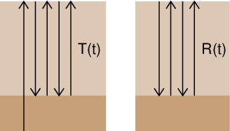
図1. このプログラムで考える地震波伝播の模式図。
Fig. 1. A schematic image for the seismic wave propagation assumed in this program.

Maeda and Watanabe (2022)ではこの手法で得られる反射応答の誤差レベルの評価手法を考案した。観測波形$u_i^{obs}(t)$はイベントによる真のシグナル $u_{i,j}^{eq}(t)$とランダムノイズ $u_{i,j}^{noise}(t)$ の重ね合わせとして \[\begin{equation} u_i^{obs}(t)=u_{i,j}^{eq}(t)+u_{i,j}^{noise}(t) \label{eq.obs} \end{equation}\] と書けると仮定する。もし何らかの方法で$u_{i,j}^{noise}(t)$を推定することができれば、 (\ref{eq.obs})式を変形した \[\begin{equation} u_{i,j}^{eq}(t)=u_i^{obs}(t)-u_{i,j}^{noise}(t) \label{eq.subtract_noise} \end{equation}\] によってランダムノイズを含まない「真のイベント波形」を得ることができ、その自己相関関数 \[\begin{equation} \textcolor[rgb]{0,0.5,0}{a_{i,j}^{eq}(\tau)}= \frac{\int u_{i,j}^{eq}(t)u_{i,j}^{eq}(t+\tau)dt} {\int u_{i,j}^{eq}(t)^2 dt} \label{eq.a} \end{equation}\] が「真の自己相関関数」となる。実際には$u_{i,j}^{noise}(t)$を推定することはできないが、その大きさだけは見積もることができる。イベント到着前後でランダムノイズの大きさが変化しないと仮定すれば、イベント到着前のタイムウインドウの波形の標準偏差 $\sigma_i^{obs}$を $u_{i,j}^{noise}(t)$の振幅レベルと見なせる。そこで平均が0で標準偏差が$\sigma_i^{obs}$のランダムノイズ波形を $N_{random}$通り生成し、これらを$u_{i,j}^{noise}(t)$の候補として (\ref{eq.subtract_noise})(\ref{eq.a})式を適用することで $u_{i,j}^{eq}(t)$, $a_{i,j}^{eq}(\tau)$の候補を $N_{random}$通り生成する。これはもちろんランダムノイズの影響を除去するという意味ではなく(除去はできない)、ランダムノイズが含まれることによって観測波形やそこから推定される自己相関関数の各データサンプルにどの程度の不確定性が含まれうるかを推定するという意味である。 $u_{i,j}^{eq}(t)$や$a_{i,j}^{eq}(\tau)$の下付き添字の$j$はランダムノイズ番号を表しており、$j=1,2,\cdots,N_{random}$である。 $a_{i,j}^{eq}(\tau)$の$j$に関する平均値を $a_i^{ave}(\tau)$、標準偏差を$\sigma_i^a(\tau)$とすると、これらが自己相関関数の最尤推定値と誤差レベルを表す。
Maeda and Watanabe (2022) developed a method to estimate the error levels in the reflection response obtained by this approach. Suppose that the observed waveform $u_i^{obs}(t)$ is a superposition of the true event signal $u_{i,j}^{eq}(t)$ and a random noise $u_{i,j}^{noise}(t)$, as expressed in Eq. (\ref{eq.obs}). If $u_{i,j}^{noise}(t)$ could be investigated in some way, Eq. (\ref{eq.obs}) can be arranged as (\ref{eq.subtract_noise}) to compute a “true (noise-free) event waveform”, and the ACF of it (Eq. \ref{eq.a}) would be a “true ACF”. Indeed, it is impossible to estimate $u_{i,j}^{noise}(t)$; however, the magnitude of it can be estimated. Assuming that the magnitude of random noise is invariant before and after the event arrival, the standard deviation $\sigma_i^{obs}$ of the waveform in a time window before the event arrival is regarded as an amplitude level of $u_{i,j}^{noise}(t)$. Based on this idea, the program generates $N_{random}$ random noise waveforms with zero average and a standard deviation $\sigma_i^{obs}$; these random waveforms are treated as candidates of $u_{i,j}^{noise}(t)$, for which Eqs. (\ref{eq.subtract_noise}) and (\ref{eq.a}) are pplied, to create $N_{random}$ traces of $u_{i,j}^{eq}(t)$ and $a_{i,j}^{eq}(\tau)$. Of course this procedure does not mean to remove the effect of noise (the noise removal is impossible) but is to evaluate the uncertainty in each data sample of the observed waveform and ACF caused by the random noise. The subscript $_j$ in $u_{i,j}^{eq}(t)$ and $a_{i,j}^{eq}(\tau)$ represents a random noise number ($j=1,2,\cdots,N_{random}$). An average ($a_i^{ave}(\tau)$) and a standard deviation ($\sigma_i^a(\tau)$) of $a_{i,j}^{eq}(\tau)$ with respect to $j$ are the most likelihood value and error level of the ACF, respectively.

これまでは1つのイベント$i$を考えてきた。利用できるイベントが複数ある場合、分散で重み付けした平均値 \[\begin{equation} \textcolor[rgb]{0,0.5,0}{a^{ave}(\tau)}= \frac{\sum_i \frac{a_i^{ave}(\tau)}{\sigma_i^a(\tau)^2}} {\sum_i \frac{1}{\sigma_i^a(\tau)^2}} \label{eq.weighted_ave} \end{equation}\] および標準偏差 \[\begin{equation} \textcolor[rgb]{0,0.5,0}{\sigma^a(\tau)}= \frac{1}{\sqrt{\sum_i \frac{1}{\sigma_i^a(\tau)^2}}} \label{eq.weighted_stddev} \end{equation}\] をその観測点における自己相関関数の最尤推定値および誤差レベルと見なす。なお、解析は観測点ごとに完全に独立であるので観測点番号を表す添字は数式中では用いていない。
The discussion so far assumed a single event $i$. If multiple events are available, an average (Eq. \ref{eq.weighted_ave}) and a standard deviation (Eq. \ref{eq.weighted_stddev}) weighted by the variance are used for the most likelihood value and error level of the ACF at this station. In these formula, no subscript or superscript is used for the station because the analyses for different stations are completely independent.

reflection_response_eventコマンドでは各イベント・各観測点の波形$u_i^{obs}(t)$を Seismic Analysis Code (SAC)の時系列データとして与える必要がある。これ以外に各SACデータにおけるイベント信号の到着時刻一覧をテキストファイルとして用意する必要がある。テキストファイルに書かれたイベント信号の到着時刻を $t_{arriv}$として、 [$t_{arriv}+$$T_b^{noise}$, $t_{arriv}+$$T_e^{noise}$] のタイムウインドウ(ノイズウインドウ)でランダムノイズの振幅レベル$\sigma_i^a(\tau)$の計算が行われ、 [$t_{arriv}+$$T_b^{signal}$, $t_{arriv}+$$T_e^{signal}$] のタイムウインドウ(シグナルウインドウ)で自己相関関数の計算(\ref{eq.a}式の積分)が行われる ($T_b^{noise}$, $T_e^{noise}$, $T_e^{signal}$, $T_e^{signal}$ はユーザ定義の定数)。その上で観測点毎に全てのイベントについて平均した自己相関関数$a^{ave}(\tau)$(\ref{eq.weighted_ave}式) とその標準偏差$\sigma^a(\tau)$(\ref{eq.weighted_stddev}式) の計算が行われる。最後に$a^{ave}(\tau)$を (\ref{eq.Claerbout})式の$T(t)∗T(-t)$であると見なして反射応答$R(t)$の計算が行われる。その際に(\ref{eq.Claerbout})式の右辺の$\delta(t)$としてはディラックの$\delta$関数そのものではなく、観測波形に対して適用したバンドパスフィルターの効果を考慮した $\delta$関数のフィルター応答が用いられる。
The reflection_response_event command requires the waveform for each event and each station ($u_i^{obs}(t)$) as a time series data in Seismic Analysis Code (SAC) format. An additional text file is needed, which lists the arrival times of event signals in the individual SAC data. Based on the arrival time $t_{arriv}$ written in this file, the amplitude level $\sigma_i^a(\tau)$ of the random noise is computed in a time window [$t_{arriv}+$$T_b^{noise}$, $t_{arriv}+$$T_e^{noise}$] (noise window) and the computation of the ACF (the integration of Eq. \ref{eq.a}) is conducted using a time window [$t_{arriv}+$$T_b^{signal}$, $t_{arriv}+$$T_e^{signal}$] (signal window), where $T_b^{noise}$, $T_e^{noise}$, $T_e^{signal}$, and $T_e^{signal}$ are constants defined by the user. The ACFs obtained in this way from all events are then averaged to compute $a^{ave}(\tau)$(Eq. \ref{eq.weighted_ave}) and the standard deviation $\sigma^a(\tau)$(Eq. \ref{eq.weighted_stddev}). The program regards $a^{ave}(\tau)$ to be $T(t)∗T(-t)$ in Eq. (\ref{eq.Claerbout}) to compute the reflection response $R(t)$. In this step, not the Dirac $\delta$ function but its response to the band-pass filter that was applied to the observed waveforms is used.

◆ソースコード(Source code)

$YMAEDA_OPENTOOL_DIR/structural_survey/src/reflection_response_event.c

◆使用方法(Usage)

コマンドライン引数でパラメータを指定する。パラメータの一覧を下表に示す。
Specify parameters by command-line arguments. The table below shows a list of parameters.

●「-」から始まらない引数 (Arguments not beginning with “-”)

このコマンドでは「-」から始まらない引数は存在しない。
This command does not have arguments not beginning with “-”.

●1つの「-」から始まる引数 (Arguments beginning with a single “-”)

このコマンドでは1つの「-」から始まる引数は存在しない。
This command does not have arguments beginning with a single “-”.

●「--パラメータ名=パラメータ値」の形式の引数 (Arguments of a form “--Parameter name=Parameter Value”)

「--パラメータ名=パラメータ値」の形式の引数は自由な順番で指定できる。「-」から始まらない引数の間に挿入しても良い。相反する指定がなされた場合には後の指定が優先される。デフォルト値を持つパラメータは省略できる。
Arguments of a form “--Parameter name=Parameter Value” can be placed in an arbitrary order. They can even be inserted between arguments not beginning with “-”. In case of conflicting options being specified, the latter option has a higher priority. Parameters that have default values can be omitted.

パラメータ名 Parameter name	意味 Meaning	可能なパラメータ値 Allowed parameter values	デフォルト値 Default value
datadir	観測に用いる地震波形が保存されているディレクトリパス。 A directory path in which the seismograms to use are stored. このディレクトリの下にイベント毎のサブディレクトリを作り、その下に各観測点の波形データを置く。 Under this directory, create a subdirectory for each event; in each subdirectory, place the waveform data from individual stations. 波形データはSeismic Analysis Code (SAC)形式とし、ファイル名の拡張子を「.sac」とする。全てのデータでサンプリングレートが等しくなければならない。 The waveform data must be in Seismic Analysis Code (SAC) format. The file name must end with an extention “.sac”. The sampling rates for all data must be equal. 同じファイル名の波形が同じ観測点の波形であると見なして重み付きスタッキング (\ref{eq.weighted_ave}, \ref{eq.weighted_stddev}式) が適用されるので、観測点毎に共通のファイル名を用いること。例えば観測点コード、あるいは観測点・成分コードをファイル名とするのが良い。 Because the weighted stacking (Eqs. \ref{eq.weighted_ave} and \ref{eq.weighted_stddev}) is applied to waveforms in the files that have the same name, use a common file name for each station; a recommended file name is a station code, or a station code followed by a component code. バンドパスフィルターはプログラム内で自動的に適用されるので波形データとしては生波形を用意すること。 Prepare raw waveforms, as the band-pass filter is automatically applied within the program. このディレクトリ内にある全てのSACファイルが無条件に用いられるのではなく、走時リストファイル(パラメータtraveltime_list_file)内でイベント信号の到着時刻が与えられているファイルのみが用いられる。 Not all SAC files in this directory may be used; only the data that have arrival times of the event signal, given in the traveltime list file (parameter traveltime_list_file), are used.	ディレクトリ名を表す文字列。 A string that represents a directory name.	省略不可 Cannot be omitted
traveltime_list_file	各イベント・各観測点の波形におけるイベントの信号の到着時刻のリストファイル (走時リストファイル)名。 The name of a file in which the arrival time of the event signal in the waveform for each event and station are listed (traveltime list file). このファイルには1行につき1つの到着時刻を書く。各行は3列から成り、第1列: イベント名 (パラメータdatadirで指定したディレクトリの下のサブディレクトリ名) 第2列: 使用するSACファイル名からディレクトリパスと拡張子の「.sac」を除いた部分 (観測点コードなど) 第3列: そのSACファイルにおけるイベント信号の到着時刻[s] とする。列の区切りにはタブを使用する。空行と各行の#から後の部分はコメントとして無視されるので自由に挿入して良い。 In this file, write information for an arrival time in each line, composed of the following three columns: the 1st column is an event name (the subdirectory name under the directory specified by parameter datadir); the 2nd column is a SAC file name without the directory path and the extension “.sac” (which may represent, for example, a station code); and the 3rd column is the arrival time of the event signal in this SAC file. Use tabs to separate the columns. Empty lines and string after # in each line are ignored as comments. 第3列の値(イベント信号の到着時刻)は波形データにおけるサンプル時刻と一致していなければならない。また、第3列の値を文字列のbad (解析に用いるには適さない波形記録という意味) とすることができ、この値を与えたデータは解析に用いられない。 The value of the 3rd column (the arrival time of the event signal) must be identical to a sample time in the waveform data. Also, a string bad is available for the value of the 3rd column, which means that the waveform record is not good for analysis; data with this value are skipped in the analysis.	ファイル名を表す文字列。 A string that represents a file name.	省略不可 Cannot be omitted
outputdir	解析結果の出力先ディレクトリ名。 Name of the directory to output the results.	ディレクトリ名を表す文字列。 A string that represents a directory name.	省略不可 Cannot be omitted
Nrandom	使用するランダムノイズ波形の個数($N_{random}$)。 The number of random noise traces to use ($N_{random}$).	2以上の自然数。 A natural number ($\geq 2$).	1000
T_b_signal	パラメータ$T_b^{signal}$の値[s]。イベント信号の到着時刻を$t_{arriv}$として [$t_{arriv}+T_b^{signal}$, $t_{arriv}+T_e^{signal}$] のタイムウインドウ(シグナルウインドウ)が自己相関関数の計算に用いられる。 The value of parameter $T_b^{signal}$ [s]; the ACF is computed using data in a time window [$t_{arriv}+T_b^{signal}$, $t_{arriv}+T_e^{signal}$] (a signal window), where $t_{arriv}$ is the arrival time of the event signal.	波形データのサンプル間隔の整数倍となる実数($\leq 0.0$)。 A real number ($\leq 0.0$), which is an integer multiple of the sampling interval of the waveform data.	-0.5
T_e_signal	パラメータ$T_e^{signal}$の値[s]。イベント信号の到着時刻を$t_{arriv}$として [$t_{arriv}+T_b^{signal}$, $t_{arriv}+T_e^{signal}$] のタイムウインドウ(シグナルウインドウ)が自己相関関数の計算に用いられる。 The value of parameter $T_e^{signal}$ [s]; the ACF is computed using data in a time window [$t_{arriv}+T_b^{signal}$, $t_{arriv}+T_e^{signal}$] (a signal window), where $t_{arriv}$ is the arrival time of the event signal.	波形データのサンプル間隔の整数倍となる正の実数。 A positive real number, which is an integer multiple of the sampling interval of the waveform data.	9.5
T_b_noise	パラメータ$T_b^{noise}$の値[s]。イベント信号の到着時刻を$t_{arriv}$として [$t_{arriv}$ $+$ $T_b^{noise}$, $t_{arriv}$ $+$ $T_e^{noise}$] のタイムウインドウ(ノイズウインドウ)が波形のノイズレベルの評価に用いられる。 The value of parameter $T_b^{noise}$ [s]; the noise level of each waveform is evaluated in a time window [$t_{arriv}$ $+$ $T_b^{noise}$, $t_{arriv}$ $+$ $T_e^{noise}$] (a noise window), where $t_{arriv}$ is the arrival time of the event signal.	波形データのサンプル間隔の整数倍となる負の実数。 A negative real number, which is an integer multiple of the sampling interval of the waveform data.	$T_e^{noise}-$$(T_e^{signal}$$-T_b^{signal})$
T_e_noise	パラメータ$T_e^{noise}$の値[s]。イベント信号の到着時刻を$t_{arriv}$として [$t_{arriv}+T_b^{noise}$, $t_{arriv}+T_e^{noise}$] のタイムウインドウ(ノイズウインドウ)が波形のノイズレベルの評価に用いられる。 The value of parameter $T_e^{noise}$ [s]; the noise level of each waveform is evaluated in a time window [$t_{arriv}+T_b^{noise}$, $t_{arriv}+T_e^{noise}$] (a noise window), where $t_{arriv}$ is the arrival time of the event signal.	波形データのサンプル間隔の整数倍となる負の実数($>T_b^{noise}$)。 A negative real number ($>T_b^{noise}$), which is an integer multiple of the sampling interval of the waveform data.	$T_b^{signal}$
taper_st	シグナルウインドウの先頭部に掛けるtaperの長さ $T_{taper}^{st}$[s]。 [$t_{arriv}+T_b^{signal}$, $t_{arriv}+T_b^{signal}+T_{taper}^{st}$] の範囲にcosineテーパーが用いられる。 Length of the taper at the beginning part of the signal window $T_{taper}^{st}$ [s]; a cosine taper is applied to a time window [$t_{arriv}+T_b^{signal}$, $t_{arriv}+T_b^{signal}+T_{taper}^{st}$].	波形データのサンプル間隔の整数倍となる非負の実数 (<$(T_e^{signal}-T_b^{signal})/2$)。 A non-negative real number (<$(T_e^{signal}-T_b^{signal})/2$), which is an integer multiple of the sampling interval of the waveform data.	$\|T_b^{signal}\|$
taper_en	シグナルウインドウの末尾部に掛けるtaperの長さ $T_{taper}^{en}$[s]。 [$t_{arriv}+T_e^{signal}-T_{taper}^{en}$, $t_{arriv}+T_e^{signal}$] の範囲にcosineテーパーが用いられる。 Length of the taper at the end part of the signal window $T_{taper}^{en}$ [s]; a cosine taper is applied to a time window [$t_{arriv}+T_e^{signal}-T_{taper}^{en}$, $t_{arriv}+T_e^{signal}$].	波形データのサンプル間隔の整数倍となる非負の実数 (< $(T_e^{signal}-T_b^{signal})/2$)。 A non-negative real number (< $(T_e^{signal}-T_b^{signal})/2$), which is an integer multiple of the sampling interval of the waveform data.	$T_{taper}^{st}$
Nsamples_whitening	スペクトルの白色化に用いるサンプル数 ($N_{samples}^{whitening}$)。周波数領域において各サンプルの値をそのサンプルを中心とする$N_{samples}^{whitening}$サンプルの絶対値平均で割ることによって白色化する。 The number of samples used for a spectral whitening ($N_{samples}^{whitening}$); each sample in a frequency domain is divided by the absolute value average of $N_{samples}^{whitening}$ samples centered on the frequency to whiten the spectrum.	正の奇数。 A positive odd number.	11
hpc	使用するバンドパスフィルターのハイパス(低周波)側のコーナー周波数[Hz]。 The corner frequency [Hz] at the high-pass (low-frequency) side of the band-pass filter to be applied.	正の実数。 A positive real number.	省略不可 Cannot be omitted
hpn	使用するバンドパスフィルターのハイパス(低周波)側の極の数。最小位相フィルターを時間の順方向と逆方向に1回ずつ掛けることによってゼロ位相フィルターを実現するが、パラメータhpnでは最小位相フィルター1回あたりの極の数を指定する。 The number of poles at the high-pass (low-frequency) side of the band-pass filter to be applied. A zero-phase filter is realized by sequentially applying minimum phase filters in normal and reversed orders of time, and parameter hpn indicates the number of poles in each minimum phase filter.	正の整数。 A positive integer.	2
lpc	使用するバンドパスフィルターのローパス(高周波)側のコーナー周波数[Hz]。 The corner frequency [Hz] at the low-pass (high-frequency) side of the band-pass filter to be applied.	パラメータhpcよりも大きな正の実数。 A positive real number greater than parameter hpc.	省略不可 Cannot be omitted
lpn	使用するバンドパスフィルターのローパス(高周波)側の極の数。最小位相フィルターを時間の順方向と逆方向に1回ずつ掛けることによってゼロ位相フィルターを実現するが、パラメータlpnでは最小位相フィルター1回あたりの極の数を指定する。 The number of poles at the low-pass (high-frequency) side of the band-pass filter to be applied. A zero-phase filter is realized by sequentially applying minimum phase filters in normal and reversed orders of time, and parameter lpn indicates the number of poles in each minimum phase filter.	正の整数。 A positive integer.	2
SNratio_min	解析に使用するシグナル/ノイズ比の下限。シグナルウインドウでの標準偏差とノイズウインドウでの標準偏差の比がこの値を下回る波形は解析に使用しない。 The lower limit of a signal-to-noise ratio to use a waveform for the analysis. A waveform is not used for the analysis if the ratio of standard deviations in the signal window to the noise window is less than this value.	非負の実数。0.0を指定すれば下限無しとなる。 A non-negative real number; 0.0 results in no lower limit.	1.0
output_filtered_impulse	$\delta$関数のフィルター応答波形(filtered_impulse.seq2) の出力の有無。 Whether to output the filter response waveform of $\delta$ function (filtered_impulse.seq2).	yes 出力する。 Output. no 出力しない。 Do not output.	yes
output_individual_event_results	個々のイベント毎の反射応答の出力の有無。 Whether to output the reflection responses from individual events.	yes 出力する。 Output. no 出力しない。 Do not output.	yes
verbose	進行状況の表示の有無。 Whether to display the progress.	yes 進行状況を表示する。 Display the progress. no 進行状況を表示しない。 Do not display the progress.	yes

◆動作(Behaviour)

Maeda and Watanabe (2022)の方法で反射応答とその標準偏差を計算し、パラメータoutputdirで指定したディレクトリに結果を出力する。
Compute the reflection response and its standard deviation based on the method of Maeda and Watanabe (2022) and output the results to a directory specified by parameter outputdir.

出力ディレクトリにはfiltered_impulse.seq2と観測点毎のサブディレクトリが作成される。
In the output directory, filtered_impulse.seq2 and subdirectories for stations are created.
filtered_impulse.seq2には (\ref{eq.Claerbout})式を用いて自己相関関数を反射応答に変換する際に用いられた $\delta$関数のフィルター応答が出力される。 ymaeda_opentoolsの時系列データ用ファイル形式 (独自のファイル形式参照) の1つであるseq2形式となる。
In filtered_impulse.seq2, the filter response of a $\delta$ function used to convert ACFs to reflection responses based on Eq. (\ref{eq.Claerbout}) are written in seq2 format, which is a file format for time series data in ymaeda_opentools; see Special file format.

なお、パラメータoutput_filtered_responseの値がnoの場合はこのファイルは出力されない。
This file is not created when the value of parameter output_filtered_response is no.
観測点毎のサブディレクトリ名には走時リストファイルの第2列の値が用いられる。
For the subdirectory name for each station, the corresponding value in the 2nd column of the traveltime list file is used.
観測点毎のサブディレクトリにはイベント毎の解析結果(イベント名.dat)とそれらを(\ref{eq.weighted_ave})(\ref{eq.weighted_stddev})式に基づいてスタッキングした結果(stack.dat)が出力される。イベント名は走時リストファイルの第1列の値である。
In the subdirectory for each station, results from each event (event name.dat) and results from stacking them based on Eqs. (\ref{eq.weighted_ave}) and (\ref{eq.weighted_stddev}) (stack.dat) are created, where event name is the corresponding value in the 1st column of the traveltime list file.

なお、パラメータoutput_individual_event_resultsの値がnoの場合はイベント名.datは出力されない。
Files event name.dat are not created when the value of parameter output_individual_event_results is no.
イベント名.datにおいては第1列がラグタイム$\tau$、第2列が$a_i^{ave}(\tau)$を元に計算される反射応答の期待値$R_i^{ave}(\tau)$、第3列が反射応答の標準偏差$\sigma_i^a(\tau)$、第4列が比$R_i^{ave}(\tau)/\sigma_i^a(\tau)$である。
In the event name.dat, the 1st column is the lag time $\tau$, the 2nd column is the expected value of the reflection response $R_i^{ave}(\tau)$ computed from $a_i^{ave}(\tau)$, the 3rd column is the standard deviation $\sigma_i^a(\tau)$ of the reflection response, and the 4th column is the ratio $R_i^{ave}(\tau)/\sigma_i^a(\tau)$.
stack.datにおいては第1列がラグタイム$\tau$、第2列が$a^{ave}(\tau)$を元に計算される反射応答の期待値$R^{ave}(\tau)$、第3列が反射応答の標準偏差$\sigma^a(\tau)$、第4列が比$R^{ave}(\tau)/\sigma^a(\tau)$である。
In the stack.dat, the 1st column is the lag time $\tau$, the 2nd column is the expected value of the reflection response $R^{ave}(\tau)$ computed from $a^{ave}(\tau)$, the 3rd column is the standard deviation $\sigma^a(\tau)$ of the reflection response, and the 4th column is the ratio $R^{ave}(\tau)/\sigma^a(\tau)$.

◆使用例(Example)

reflection_response_event --datadir=../data/sacfiles --traveltime_list_file=traveltimes.dat --outputdir=results --hpc=1.0 --lpc=10.0

●../data/sacfilesの中身 (Files in ../data/sacfiles)

event1/station1.sac
event1/station2.sac
event1/station3.sac
event1/station4.sac

event2/station1.sac
event2/station2.sac
event2/station3.sac
event2/station5.sac

event3/station2.sac
event3/station3.sac
event3/station4.sac
event3/station5.sac

event4/station3.sac
event4/station4.sac

●traveltimes.datの中身 (Content in traveltimes.dat)

#event1 (no data for station3)
event1[TAB]station1.sac[TAB]12.3
event1[TAB]station2.sac[TAB]12.4
event1[TAB]station4.sac[TAB]13.5

#event2
event2[TAB]station1.sac[TAB]14.1
event2[TAB]station1.sac[TAB]bad
event2[TAB]station3.sac[TAB]14.0
event2[TAB]station5.sac[TAB]13.8

#event3
event3[TAB]station2.sac[TAB]20.1
event3[TAB]station3.sac[TAB]20.2
event3[TAB]station4.sac[TAB]20.0
event3[TAB]station5.sac[TAB]20.3

#event4
event4[TAB]station3.sac[TAB]15.0
event4[TAB]station4.sac[TAB]14.5

ここで[TAB]はタブを表す。 event1/station3.sacは波形データは存在するがこのファイルで走時が与えられていないので解析に用いられない。 event2/station2.sacは第3列の値がbadになっているので解析に用いられない。
Here, [TAB] indicates a tab. File event1/station3.sac is not used for the analysis because of absence of the traveltime in this file. File event2/station2.sac is not used because the value of the 3rd column is “bad”.

●この例において出力されるファイル (Output files in this example)

results/filtered_impulse.seq2

results/station1/event1.dat
results/station1/event2.dat
results/station1/stack.dat

results/station2/event1.dat
results/station2/event3.dat
results/station2/stack.dat

results/station3/event2.dat
results/station3/event3.dat
results/station3/event4.dat
results/station3/stack.dat

results/station4/event1.dat
results/station4/event3.dat
results/station4/event4.dat
results/station4/stack.dat

results/station5/event2.dat
results/station5/event3.dat
results/station5/stack.dat

◆引用文献 (References)

★ は本プログラムを用いた研究成果の発表時に必ず引用すべき論文を表す。
The star (★) indicates the references that must be cited whenever a research that used this program is published or presented.

Claerbout JF (1968) Synthesis of a layered medium from its acoustic transmission response, Geophysics 33(2), 264-269. https://doi.org/10.1190/1.1439927
★ Maeda Y, Watanabe T (2022) Estimating errors in autocorrelation functions for reliable investigations of reflection profiles, Earth Planets Space 74, 48. https://doi.org/10.1186/s40623-022-01606-5

reflection_response_eventコマンド マニュアル