waterPMLコマンドの検証

5. 水域を用いた計算

(Examples and validations for waterPML command — 5. computation using water-filled regions)


◆概要と問題設定 (Outline and the problem)

waterPMLコマンドを用いた計算の5つ目の例として水域を含んだ計算を試してみる。 このサイトで公開可能な地形データが存在しないので人工的に作成した地形データを用いる。 地形は異なるが、ここではMaeda and Kumagai (2013)の図5の特徴の再現を目標とし、 図1に示す地形データ、水域、地震波動ソース、観測点を用いる。 1つ目の観測点は地震波動ソースと同じ島内に位置しており、 そこでの波形は火口湖の影響のみを受ける。 2つ目の観測点は遠方に位置しており、伝播経路の大部分が水域を含んでいる。
The 5th example of computation with the waterPML command uses water-filled regions. There is no real topography data that can be opened in this website. Therefore, an artificial topography data is used. Fig. 1 shows the topography, water-filled regions, the seismic wave source, and stations used in this example. The goal of this simulation is to reproduce the characteristics in Fig. 5 of Maeda and Kumagai (2013), although the topography is different. The 1st station is located in the same island as the seismic wave source, so that the waveforms at this station is affected only by the crater lake. The 2nd station is distant, and most of the propagation path from the source to this station includes water-filled regions.


図1. 問題設定。(a)水平面、(b)\(y=0\)の鉛直断面。 地形を(a)に色と等値線(100 m間隔)で、(b)に茶色で示す。 水域を(a)に太線で、(b)に水色で示す。 は地震波動ソースの位置、 ▲は観測点の位置を表す。
Fig. 1. The problem to be solved in (a) horizontal section and (b) a vertical section along \(y=0\). The topography is shown by color scale and contours (100 m intervals) in Fig. 1a and brown in Fig. 1b. Water-filled regions are shown by thick lines in Fig. 1a and blue in Fig. 1b. The star () and triangles () indicate the locations of the seismic wave source and stations, respectively.


◆地形 (Topography)

以下の関数形で表される地形を使用する。
Eq. (\ref{eq.topography}) is the topography used in this example.

\[\begin{eqnarray} h(x,y) &=& -D +h_1 \exp\left[-\frac{(x-x_1)^2+y^2}{r_{1m}^2}\right] -d_1 \exp\left[-\frac{(x-x_1)^2+y^2}{r_{1c}^2}\right] \nonumber \\ & & +h_2 \exp\left[-\frac{(x-x_2)^2+y^2}{r_{2m}^2}\right] \label{eq.topography} \end{eqnarray}\]
(\ref{eq.topography})式のパラメータは表1のように設定する。
Parameters in Eq. (\ref{eq.topography}) are listed in Table 1.

表1. (\ref{eq.topography})式のパラメータ。
Table 1. Parameters in Eq. (\ref{eq.topography}).
パラメータ
Parameter

Value
\(D\) 300 m
\(h_1\) 900 m
\(d_1\) 700 m
\(h_2\) 600 m
\(r_{1m}\) 2000 m
\(r_{1c}\) 400 m
\(r_{2m}\) 1000 m
\(x_1\) -5500 m
\(x_2\) 5500 m

(\ref{eq.topography})式は 深さ\(D\)の海底から2つの山体が盛り上がる地形を表している。 1つ目の山体は位置\((x_1,0)\)を中心とする 比高\(h_1\)、水平距離スケール\(r_{1m}\)の山体であり、 その中央に深さ\(d_1\)、水平距離スケール\(r_{1c}\)の凹みがある。 2つ目の山体は位置\((x_2,0)\)を中心とする 比高\(h_2\)、水平距離スケール\(r_{2m}\)の山体である(図1)。 この地形データを作成するコマンドを以下に示す。
Eq. (\ref{eq.topography}) represents a topography that consists of two mountains from the seafloor of depth \(D\). The 1st mountain has a relative height \(h_1\) and a horizontal length scale \(r_{1m}\) centered on \((x_1,0)\). A crater of depth \(d_1\) and a horizontal length scale \(r_{1c}\) is located at the center of this mountain. The 2nd mountail has a relative height \(h_2\) and a horizontal length scale \(r_{2m}\) (Fig. 1). A command to create this topography data is shown below.

rm -f topography_ex5.dat
for((x=-7100;x<=7100;x+=100))
do
  for((y=-3100;y<=3100;y+=100))
  do
    echo $x $y | awk '{ D=300.0; h1=900.0; d1=700.0; h2=600.0; r1m=2000.0; r1c=400.0; r2m=1000.0; x1=-5500.0; x2=5500.0; distance1_2=($1-x1)*($1-x1)+$2*$2; distance2_2=($1-x2)*($1-x2)+$2*$2; h=-D; if(distance1_2<100.0*r1m*r1m){ h+=h1*exp(-distance1_2/(r1m*r1m)); } if(distance1_2<100.0*r1c*r1c){ h-=d1*exp(-distance1_2/(r1c*r1c)); } if(distance2_2<100.0*r2m*r2m){ h+=h2*exp(-distance2_2/(r2m*r2m)); } printf("%d\t%d\t%f\n",$1,$2,h); }' >> topography_ex5.dat
  done
done

ここで警告を避けるためにexpの中身が-100よりも大きい場合のみ 各項を加算するように場合分けした。
Here, each term is added only if the content of exp is greater than -100 to avoid warning.


●水域 (Water-filled regions)

標高0 mに海面を置く。 また、1つ目の山の中央の火口において標高300 mに水面を置く(図1)。 これらの水域を表現するためのwaterPMLコマンド用の設定ファイルを以下に示す。
The sea surface is placed at an elevation of 0 m. The crater of the first mountain is filled with a lake that has a water surface of 300 m above sea level (Fig. 1). A configuration file for waterPML command to express these water-filled regions is shown below.

(water5.ini)
newlake sea
height=0.0

newlake crater_lake
height=300.0
xmin=-6000.0
xmax=-5000.0
ymin=-500.0
ymax=500.0


●地震波動ソース (Seismic wave source)

Maeda and Kumagai (2013)にならって 時定数\(\tau_p=1\) s, \(\tau_s=2\) sのリッカー波を 震源時間関数として用いる。 火口湖の下の浅部(図1)における等方ソースとする。 waterPMLコマンド用の地震波動ソースの設定ファイルは以下のようになる。
Following Maeda and Kumagai (2013), a Ricker wavelet with time constants \(\tau_p=1\) s and \(\tau_s=2\) s is used as the source time function. An isotropic source at a shallow depth beneath the crate lake (Fig. 1) is used. The configuration file of this seismic wave source for the waterPML command is as below.

(source5.ini)
newsource isotropic
location_x=-5500.0
location_y=0.0
location_z=-450.0
mechanism=isotropic
intensity=1.0
stfun_name=ricker
stfun_tp=1.0
stfun_ts=2.0


●観測点 (Stations)

冒頭で述べたように、地震波動ソースと同じ島内に1点、水域を挟んだ遠方に1点の 計2つの観測点を使用する。 waterPMLコマンド用の観測点リストファイルを以下に示す。
Two stations are used, as have been described at the beginning of this page. One station is located in the same island as the seismic wave source, and the other is located at a large distance from the source, between which a water-filled region is present. A station list file for the waterPML command is shown below.

(station_list5.dat)
NEAR[TAB]-4600.0[TAB]0.0[TAB]surface-0.1
FAR[TAB]4900.0[TAB]0.0[TAB]surface-0.1


●問題設定のプロット (Plotting the problem setting)

waterPMLコマンドを実行する上で必須ではないが、 Generic Mapping Tools (version 6) を用いて図1をプロットするコマンドを以下に示す。
Although it is not required for running waterPML, commands to generate Fig. 1 by Generic Mapping Tools (version 6) are shown below.

gmt begin problem5 ps

gmt set FONT_ANNOT_PRIMARY 12p

#地形のプロット(水平面)
#Plotting topography in horizontal section
gmt surface topography_ex5.dat -R-7100/7100/-3100/3100 -I100/100 -Gtopography_ex5.grd

gmt makecpt -Cdrywet -T-500/500/10 -Z -I -D

gmt grdimage topography_ex5.grd -R-7100/7100/-3100/3100 -JX14.2/6.2 -Xa3 -Ya6

gmt grdcontour topography_ex5.grd -R-7100/7100/-3100/3100 -JX14.2/6.2 -Xa3 -Ya6 -C100 -W0.4,100/100/100

#海岸線のプロット(水平面)
#Plotting coastline in horizontal section
awk '{ if(($1+5500.0)*($1+5500.0)+$2*$2<500.0*500.0){ print $1,$2,$3-300.0 }else{ print $1,$2,$3 } }' topography_ex5.dat | gmt surface -R-7100/7100/-3100/3100 -I100/100 -Gtopography_ex5_for_coastline.grd

gmt grdcontour topography_ex5_for_coastline.grd -R-7100/7100/-3100/3100 -JX14.2/6.2 -Xa3 -Ya6 -C2000 -W2,0/0/0 -Bxa2000f1000 -Bya2000f1000 -BWsen

#水域のプロット(東西断面)
#Plotting water-filled regions in EW section
gmt plot -R-7100/7100/-2000/700 -JX14.2/2.7 -Xa3 -Ya3 -G127/191/255 <<EOF
-7100 0
7100 0
7100 -1000
-7100 -1000
>
-6000 300
-5000 300
-5000 -1000
-6000 -1000
EOF

#地形のプロット(東西断面)
#Plotting topography in EW section
awk '($2==0){ print $1,$3 } END{ printf("7100\t-2000\n"); printf("-7100\t-2000\n"); }' topography_ex5.dat | gmt plot -R-7100/7100/-2000/700 -JX14.2/2.7 -Xa3 -Ya3 -G220/180/140 -Bxa2000f1000 -Bya500f100 -BWSen

#地震波動ソースのプロット
#Plotting seismic wave source
gmt plot -R-7100/7100/-3100/3100 -JX14.2/6.2 -Xa3 -Ya6 -Sa0.4 -G255/0/0 <<EOF
-5500 0
EOF

gmt plot -R-7100/7100/-2000/700 -JX14.2/2.7 -Xa3 -Ya3 -Sa0.4 -G255/0/0 <<EOF
-5500 -450
EOF

#観測点のプロット
#Plotting stations
gmt plot -R-7100/7100/-3100/3100 -JX14.2/6.2 -Xa3 -Ya6 -St0.4 -G0/0/0 <<EOF
-4600 0
4900 0
EOF

gmt plot -R-7100/7100/-2000/700 -JX14.2/2.7 -Xa3 -Ya3 -St0.4 -G0/0/0 <<EOF
-4600 431
4900 119
EOF

#文字列のプロット
#Plotting texts
gmt text -R0/21/0/29.7 -JX21/29.7 -Xa0 -Ya0 -F+f12p+a+j <<EOF
10.1 2.2 0 CT East (m)
1.5 9.1 90 CB North (m)
1.5 4.35 90 CB Elevation (m)
17.0 5.5 0 RT (b)
EOF

gmt text -R0/21/0/29.7 -JX21/29.7 -Xa0 -Ya0 -F+f12p,,255/255/255+a+j <<EOF
17.0 12.0 0 RT (a)
EOF

gmt end


◆計算 (The calculation)

計算には以下のコマンドを用いる。
Use the command below to perform the calculation.

waterPML --Nx=141 --Ny=61 --Nz=27 --Npmx=20 --x0=-7050.0 --y0=-3050.0 --z0=-2000.0 --dx=100.0 --dt=0.01 --tmax=20.0 --topography_files=topography_ex5.dat --topography_file_format=xy --water_file=water5.ini --structure_file=structure5.ini --structure_file_format=layer --source_file=source5.ini --output_dir=result05 --station_file=station_list5.dat

ここでは物理領域を\(-7050\leq x\leq 7050\), \(-3050\leq y\leq 3050\), \(-2000\leq z\leq 700\) (単位:m, 図1)とし、格子セルサイズを100 mとした。 ファイルtopography_ex5.dat, water5.ini, source5.ini, station_list5.dat については既に説明した。 今までの例題との最大の相違点は--water_file=のオプション(赤字)を用いていることである。 地下構造(structure5.ini)はMaeda and Kumagai (2013)に合わせて P波速度\(V_p=3500\) m/s, S波速度\(V_s=V_p/\sqrt{3}=2020.7\) m/s, 密度2400 kg/m\(^3\)の均質媒質とする。
Here, the physical volume is \(-7050\leq x\leq 7050\), \(-3050\leq y\leq 3050\), \(-2000\leq z\leq 700\) (unit: m, Fig. 1) and a grid cell size is 100 m. Files topography_ex5.dat, water5.ini, source5.ini, and station_list5.dat have already been explained. The most essential difference from the previous examples is the use of --water_file= option (shown by red). The subsurface structure (structure5.ini) is a homogeneous medium with a P-wave velocity \(V_p=3500\) m/s, and S-wave velocity \(V_s=V_p/\sqrt{3}=2020.7\) m/s, and a density 2400 kg/m\(^3\) (Maeda and Kumagai 2013).

(structure5.ini)
1000.0[TAB]3500.0[TAB]2020.7[TAB]2400.0
-2500.0[TAB]3500.0[TAB]2020.7[TAB]2400.0


◆比較のための水域を含まない計算 (Computations without water-filled regions for comparison)

計算結果についてMaeda and Kumagai (2013)の図5と同様の評価を行うため、 水域を含まない計算を行う。
To evaluate the computation results in the same manner as Fig. 5 of Maeda and Kumagai (2013), let us perform computation without water-filled regions.


●水を真空で置き換えた計算 (Computation with replacing water by vacuum)

水を真空で置き換えた計算を行うには 上記のコマンドで単純に--water=fileオプションを除けば良い。 計算結果が上書きされないように出力ディレクトリを変更する。
To perform a computation using vacuum instead of water, simply remove --water_file option from the command above. Change the output directory to avoid the previous computation results from being overwritten.

waterPML --Nx=141 --Ny=61 --Nz=27 --Npmx=20 --x0=-7050.0 --y0=-3050.0 --z0=-2000.0 --dx=100.0 --dt=0.01 --tmax=20.0 --topography_files=topography_ex5.dat --topography_file_format=xy --structure_file=structure5.ini --structure_file_format=layer --source_file=source5.ini --output_dir=result05_vacuum --station_file=station_list5.dat


●水を固体で置き換えた計算 (Computation with replacing water by solid)

水を固体で置き換えた計算を行うには地形データの修正が必要である。 まず以下のコマンドで地形データ(topography_ex5_filled_with_solid.dat)を作成する。
To perform a computation using solid instead of water, the topography data needs to be modified. First, create an alternative topography data (topography_ex5_filled_with_solid.dat) by the commands below.

rm -f topography_ex5_filled_with_solid.dat
for((x=-7100;x<=7100;x+=100))
do
  for((y=-3100;y<=3100;y+=100))
  do
    echo $x $y | awk '{ D=300.0; h1=900.0; d1=700.0; h2=600.0; r1m=2000.0; r1c=400.0; r2m=1000.0; x1=-5500.0; x2=5500.0; distance1_2=($1-x1)*($1-x1)+$2*$2; distance2_2=($1-x2)*($1-x2)+$2*$2; h=-D; if(distance1_2<100.0*r1m*r1m){ h+=h1*exp(-distance1_2/(r1m*r1m)); } if(distance1_2<100.0*r1c*r1c){ h-=d1*exp(-distance1_2/(r1c*r1c)); } if(distance2_2<100.0*r2m*r2m){ h+=h2*exp(-distance2_2/(r2m*r2m)); } if(distance1_2<500.0*500.0 && h<300.0){ h=300.0; } if(h<0.0){ h=0.0; } printf("%d\t%d\t%f\n",$1,$2,h); }' >> topography_ex5_filled_with_solid.dat
  done
done

確認のため、この地形データをプロットする。
Plot this topography data for check.

gmt begin topography_ex5_filled_with_solid ps

gmt set FONT_ANNOT_PRIMARY 12p

gmt surface topography_ex5_filled_with_solid.dat -R-7100/7100/-3100/3100 -I100/100 -Gtopography_ex5_filled_with_solid.grd

gmt makecpt -Cdrywet -T-600/600/10 -Z -I -D

gmt grdimage topography_ex5_filled_with_solid.grd -R-7100/7100/-3100/3100 -JX14.2/6.2 -Xa3 -Ya6 -Bxa2000f1000 -Bya2000f1000 -BWsen

awk '($2==0){ print $1,$3 } END{ printf("7100\t-2000\n"); printf("-7100\t-2000\n"); }' topography_ex5_filled_with_solid.dat | gmt plot -R-7100/7100/-2000/700 -JX14.2/2.7 -Xa3 -Ya3 -G220/180/140 -Bxa2000f1000 -Bya500f100 -BWSen

gmt text -R0/21/0/29.7 -JX21/29.7 -Xa0 -Ya0 -F+f12p+a+j <<EOF
8.1 2.2 0 CT East (m)
1.5 9.1 90 CB North (m)
1.5 4.35 90 CB Elevation (m)
17.0 12.0 0 RT (a)
17.0 5.5 0 RT (b)
EOF

gmt end

結果を図2に示す。 図1と比べると水域を固体で置き換えた地形になっていることが分かる。
The result is shown in Fig. 2, showing that the water in Fig. 1 was replaced by solid successfully.


図2. 水域を固体で置き換えた地形。
Fig. 2. A topography where water was replaced by solid.

この地形データを用いてwaterPMLコマンドを実行する。
Execute waterPML command using this topography data.

waterPML --Nx=141 --Ny=61 --Nz=27 --Npmx=20 --x0=-7050.0 --y0=-3050.0 --z0=-2000.0 --dx=100.0 --dt=0.01 --tmax=20.0 --topography_files=topography_ex5_filled_with_solid.dat --topography_file_format=xy --structure_file=structure5.ini --structure_file_format=layer --source_file=source5.ini --output_dir=result05_solid --station_file=station_list5.dat


◆計算結果の比較 (Comparison of results)

以上で
の結果が得られた。 これらの波形をプロット用にseq2形式に変換する。
Computation results have been obtained for the following three models:
Convert these waveforms to seq2 format for plotting.

for dir in result05 result05_vacuum result05_solid
do
  cd $dir/waveform
  for station in NEAR FAR
  do
    for component in Vx Vy Vz
    do
      sequencefile_convert $station.$component seq1 seq2
    done
  done
  cd ../..
done

次に、得られた波形をプロットする。 \(y\)成分は振幅が0であるので\(x\)成分と\(z\)成分のみをプロットすれば良い。
Next, plot the \(x\)- and \(z\)-components of the waveforms; \(y\)-component is zero.

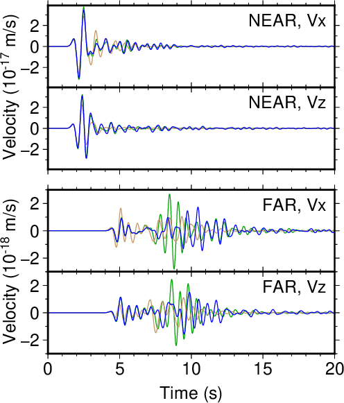
gmt begin waveforms5 ps

gmt set FONT_ANNOT_PRIMARY 12p

# NEAR, Vx
awk '(NF==2){ print $1,$2*1.0e+17 }' result05_vacuum/waveform/NEAR.Vx.seq2 | gmt plot -R0/20/-3.9/3.9 -JX7/2 -Xa3 -Ya9.5 -W0.5,0/160/0

awk '(NF==2){ print $1,$2*1.0e+17 }' result05_solid/waveform/NEAR.Vx.seq2 | gmt plot -R0/20/-3.9/3.9 -JX7/2 -Xa3 -Ya9.5 -W0.5,200/150/100

awk '(NF==2){ print $1,$2*1.0e+17 }' result05/waveform/NEAR.Vx.seq2 | gmt plot -R0/20/-3.9/3.9 -JX7/2 -Xa3 -Ya9.5 -W0.5,0/0/255 -Bxa5f1 -Bya2f1 -BWsen

# NEAR, Vz
awk '(NF==2){ print $1,$2*1.0e+17 }' result05_vacuum/waveform/NEAR.Vz.seq2 | gmt plot -R0/20/-3.9/3.9 -JX7/2 -Xa3 -Ya7.5 -W0.5,0/160/0

awk '(NF==2){ print $1,$2*1.0e+17 }' result05_solid/waveform/NEAR.Vz.seq2 | gmt plot -R0/20/-3.9/3.9 -JX7/2 -Xa3 -Ya7.5 -W0.5,200/150/100

awk '(NF==2){ print $1,$2*1.0e+17 }' result05/waveform/NEAR.Vz.seq2 | gmt plot -R0/20/-3.9/3.9 -JX7/2 -Xa3 -Ya7.5 -W0.5,0/0/255 -Bxa5f1 -Bya2f1 -BWsen

# FAR, Vx
awk '(NF==2){ print $1,$2*1.0e+18 }' result05_vacuum/waveform/FAR.Vx.seq2 | gmt plot -R0/20/-3/3 -JX7/2 -Xa3 -Ya5 -W0.5,0/160/0

awk '(NF==2){ print $1,$2*1.0e+18 }' result05_solid/waveform/FAR.Vx.seq2 | gmt plot -R0/20/-3/3 -JX7/2 -Xa3 -Ya5 -W0.5,200/150/100

awk '(NF==2){ print $1,$2*1.0e+18 }' result05/waveform/FAR.Vx.seq2 | gmt plot -R0/20/-3/3 -JX7/2 -Xa3 -Ya5 -W0.5,0/0/255 -Bxa5f1 -Bya2f1 -BWsen

# FAR, Vz
awk '(NF==2){ print $1,$2*1.0e+18 }' result05_vacuum/waveform/FAR.Vz.seq2 | gmt plot -R0/20/-3/3 -JX7/2 -Xa3 -Ya3 -W0.5,0/160/0

awk '(NF==2){ print $1,$2*1.0e+18 }' result05_solid/waveform/FAR.Vz.seq2 | gmt plot -R0/20/-3/3 -JX7/2 -Xa3 -Ya3 -W0.5,200/150/100

awk '(NF==2){ print $1,$2*1.0e+18 }' result05/waveform/FAR.Vz.seq2 | gmt plot -R0/20/-3/3 -JX7/2 -Xa3 -Ya3 -W0.5,0/0/255 -Bxa5f1 -Bya2f1 -BWSen

# text
gmt text -R0/21/0/29.7 -JX21/29.7 -Xa0 -Ya0 -F+f12p+a+j <<EOF
6.5 2.2 0 CT Time (s)
2.2 9.5 90 CB Velocity (10@+-17@+ m/s)
2.2 5.0 90 CB Velocity (10@+-18@+ m/s)
9.8 11.3 0 RT NEAR, Vx
9.8 9.3 0 RT NEAR, Vz
9.8 6.8 0 RT FAR, Vx
9.8 4.8 0 RT FAR, Vz
EOF

gmt end

プロットした波形を図3に示す。 近場の観測点においては3つの波形はよく合っており、 主な違いは振幅の違いである。 一方、遠方観測点においてはレイリー波の部分に大きな差異が見られ、 水域を用いた計算(青)ではレイリー波の最大振幅の時刻が後ろにずれている。 これらの特徴はMaeda and Kumagai (2013)と整合的である。
Fig. 3 shows the waveforms plotted by the commands shown above. At the near station, the three waveforms are generally consistent, with slight differences in amplitudes. At the distant station, the three waveforms are different especially in the Rayleigh wave portion; the time of the maximum amplitude of the Rayleigh wave is later in the computation with the water-filled regions than the other two results. These features are consistent with those described in Maeda and Kumagai (2013).


図3. 3種類の計算結果の比較。 青:水域を用いた計算。 緑:水域を真空で置き換えた計算。 茶色:水域を固体で置き換えた計算。
Fig. 3. Comparison of the three computation results. Blue: a computation with water-filled regions. Green: a computation in which the vacuum is used instead of water. Brown: a computation in which the solid is used instead of water.