waterPMLコマンドで用いている計算式

(2)離散化

(Formula used in waterPML command; (2) Discretization)


前節では微分方程式として (20)(21)式を導出した。これらを再掲すると \[\begin{equation} \rho \left(\PartialDiff{}{t}+\alpha^k\right) V_i^k = \sum_l \tau_{ik,k}^l + \delta_{k0} f_i \label{eq.motion.Vik.sumT.PML} \end{equation}\] \[\begin{equation} \left(\PartialDiff{}{t}+\alpha^l\right) \tau_{ij}^l = \sum_p C_{ijpl} \left(\sum_k V_{p,l}^k\right) \label{eq.constitutive.dTijl.sumV.PML} \end{equation}\] である。 この節ではこれらの式を Ohminato and Chouet (1997)の食い違い格子を用いて離散化する。 最終的に導出する式は (\ref{eq.Vik})(\ref{eq.Tijl})式であり、 これらが係数の定義式(\ref{eq.c0})(\ref{eq.c1})(\ref{eq.c2})とともに プログラム内で直接に利用される。
Eqs. (20) and (21) in the previous section, shown again in Eqs. (\ref{eq.constitutive.dTijl.sumV.PML}) and (\ref{eq.constitutive.dTijl.sumV.PML}) in this page, are the differential equations to be used. This section discritizes these equations using the staggered grid scheme proposed by Ohminato and Chouet (1997). The final equations are (\ref{eq.Vik}) and (\ref{eq.Tijl}), which are directly used in the program, where the coefficients are defined by Eqs. (\ref{eq.c0}), (\ref{eq.c1}) and (\ref{eq.c2}).


2-1. 使用する食い違い格子 (The staggered grid scheme used)

\(x_0\), \(x_1\), \(x_2\)方向への1格子セル分の変分ベクトルをそれぞれ \(\Delta\posx_0\), \(\Delta\posx_1\), \(\Delta\posx_2\)、 差分計算の時間刻みを\(\Delta t\)とする。 注目する格子セルの中心点の座標を\(\posx\)とする。 速度と応力の各成分はそれぞれ以下の位置・時刻で定義する(図1)。
Let \(\Delta\posx_0\), \(\Delta\posx_1\), and \(\Delta\posx_2\) be the vectors representing the movements by a grid cell size along \(x_0\), \(x_1\), and \(x_2\) directions, respectively, and let \(\Delta t\) be the time stepping of the computation. Let \(\posx\) be the center of a grid cell focused in the discussion here. The velocity and stress components are defined at the following locations and time samples, respectively (Fig. 1).


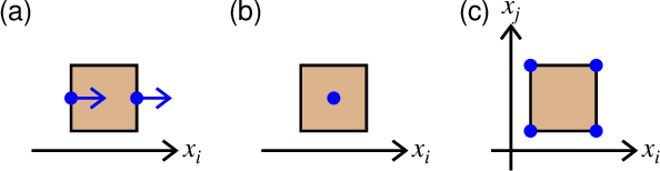
図1. 格子セルに対する変数の定義位置。 (a)速度\(V_i^k\)と等価体積力\(f_i\)、 (b)応力の対角成分\(\tau_{ii}^l\)、 (c)応力の非対角成分\(\tau_{ij}^l\), \(i\neq j\)。
Fig. 1. Definition points of variables relative to a grid cell. (a) The velocity \(V_i^k\) and equivalent body force \(f_i\), (b) diagonal stress components \(\tau_{ii}^l\), (c) off-diagonal stress components \(\tau_{ij}^l\), \(i\neq j\).


2-2. 以下で用いる記号 (Notations used below)

以下では格子セル中心点を\(\posx\)、 格子セル中心点から\(x_i\)軸の正方向に格子セルの半分だけずれた点 \(\posx+\Delta \posx_i/2\)を\(\posx_{i+1/2}\)、 \(x_j\)軸の負方向に1格子セル分ずれた点 \(\posx-\Delta \posx_j\)を\(\posx_{j-1}\)のように表す。 時刻についても同様に、時刻\(t+\Delta t/2\)を\(t_{+1/2}\)のように表す。 2つの添字が登場する場合はスペースの節約のために 一方を上付き添字で表す場合がある。 例えば\(\tau_{ik}^l\left(\posx_{i-1/2}^{k+1/2},t_{-1/2}\right)\)は \(\tau_{ik}^l(\posx-\Delta\posx_i/2+\Delta\posx_k/2,t-\Delta t/2)\) のことである。
Below, \(\posx\) is the center of a grid cell, \(\posx_{i+1/2}\) is the position obtained by a half-grid movement from the center of a grid cell to positive side in \(x_i\) direction (i.e., \(\posx+\Delta \posx_i/2\)), and \(\posx_{j-1}\) is the position obtained by a one-grid movement from the center of a grid cell to negative side in \(x_j\) direction (i.e., \(\posx-\Delta \posx_j\)). In the same way, time \(t+\Delta t/2\) is denoted as \(t_{+1/2}\). When two subscripts appear, one of them is replaced by a superscript to save the space. For example, \(\tau_{ik}^l\left(\posx_{i-1/2}^{k+1/2},t_{-1/2}\right)\) represents \(\tau_{ik}^l(\posx-\Delta\posx_i/2+\Delta\posx_k/2,t-\Delta t/2)\).


2-3. (\ref{eq.motion.Vik.sumT.PML})式の離散化 (Discretization of equation (\ref{eq.motion.Vik.sumT.PML}))

(\ref{eq.motion.Vik.sumT.PML})式の両辺に現れる偏導関数を 位置\(\posx-\Delta\posx_i/2\),時刻\(t-\Delta t/2\)のまわりの 2次精度中心差分式で近似すると \[\begin{eqnarray} \left(\PartialDiff{}{t}+\alpha^k\right) V_i^k &=& \frac{V_i^k(\posx_{i-1/2},t)-V_i^k(\posx_{i-1/2},t_{-1})}{\Delta t} \nonumber \\ & & +\alpha^k(\posx_{i-1/2}) \frac{V_i^k(\posx_{i-1/2},t)+V_i^k(\posx_{i-1/2},t_{-1})}{2} \nonumber \\ &=& \left\{\frac{1}{\Delta t}+\frac{\alpha^k(\posx_{i-1/2})}{2}\right\} V_i^k(\posx_{i-1/2},t) \nonumber \\ & & +\left\{\frac{1}{\Delta t}-\frac{\alpha^k(\posx_{i-1/2})}{2}\right\} V_i^k(\posx_{i-1/2},t_{-1}) \label{eq.motion.discretize.left} \end{eqnarray}\] \[\begin{eqnarray} \tau_{ik,k}^l &=& \frac{\tau_{ik}^l\left(\posx_{i-1/2}^{k+1/2},t_{-1/2}\right) -\tau_{ik}^l\left(\posx_{i-1/2}^{k-1/2},t_{-1/2}\right)} {|\Delta\posx_k|} \label{eq.motion.discretize.right} \end{eqnarray}\] と書ける。 但し、時刻\(t-\Delta t/2\)における\(\alpha^k V_i^k\)の値については 時刻\(t\)での値と時刻\(t-\Delta t\)での値の平均で与えられるものとした。 (\ref{eq.motion.discretize.left})(\ref{eq.motion.discretize.right}) を(\ref{eq.motion.Vik.sumT.PML})に代入すると \[\begin{eqnarray} & & \rho(\posx_{i-1/2})\left[ \left\{\frac{1}{\Delta t}+\frac{\alpha^k(\posx_{i-1/2})}{2}\right\} V_i^k(\posx_{i-1/2},t) \right. \nonumber \\ & & \left. +\left\{\frac{1}{\Delta t}-\frac{\alpha^k(\posx_{i-1/2})}{2}\right\} V_i^k(\posx_{i-1/2},t_{-1}) \right] \nonumber \\ &=& \sum_l \frac{\tau_{ik}^l\left(\posx_{i-1/2}^{k+1/2},t_{-1/2}\right) -\tau_{ik}^l\left(\posx_{i-1/2}^{k-1/2},t_{-1/2}\right)} {|\Delta\posx_k|} +\delta_{k0}f_i(\posx_{i-1/2},t_{-1/2}) \label{eq.Vik.diff1} \end{eqnarray}\] となり、この式を\(V_i^k(\posx_{i-1/2},t)\)について解くと \[\begin{eqnarray} V_i^k(\posx_{i-1/2},t) &=& \frac{\frac{1}{\Delta t}-\frac{\alpha^k(\posx_{i-1/2})}{2}} {\frac{1}{\Delta t}+\frac{\alpha^k(\posx_{i-1/2})}{2}} V_i^k(\posx_{i-1/2},t_{-1}) +\frac{1}{\rho(\posx_{i-1/2})} \frac{1}{\frac{1}{\Delta t}+\frac{\alpha^k(\posx_{i-1/2})}{2}} \nonumber \\ & & \left[ \sum_l \frac{\tau_{ik}^l\left(\posx_{i-1/2}^{k+1/2},t_{-1/2}\right) -\tau_{ik}^l\left(\posx_{i-1/2}^{k-1/2},t_{-1/2}\right)} {|\Delta\posx_k|} \right. \nonumber \\ & & \left. +\delta_{k0} f_i(\posx_{i-1/2},t_{-1/2}) \right] \label{eq.Vik.diff2} \end{eqnarray}\] が得られる。 ここで、時間依存しない係数を \[\begin{equation} c_0^k(\posx) \equiv \frac{\frac{1}{\Delta t}-\frac{\alpha^k(\posx)}{2}} {\frac{1}{\Delta t}+\frac{\alpha^k(\posx)}{2}} \label{eq.c0} \end{equation}\] \[\begin{equation} c_1^k(\posx) \equiv \frac{1}{\rho(\posx)} \frac{1}{\frac{1}{\Delta t}+\frac{\alpha^k(\posx)}{2}} \frac{1}{|\Delta\posx_k|} \label{eq.c1} \end{equation}\] とおけば \[\begin{eqnarray} V_i^k(\posx_{i-1/2},t) &=& c_0^k(\posx_{i-1/2})V_i^k(\posx_{i-1/2},t_{-1}) \nonumber \\ & & +c_1^k(\posx_{i-1/2})\left[ \sum_l \left\{\tau_{ik}^l\left(\posx_{i-1/2}^{k+1/2},t_{-1/2}\right) -\tau_{ik}^l\left(\posx_{i-1/2}^{k-1/2},t_{-1/2}\right)\right\} \right. \nonumber \\ & & \left. +\delta_{k0}|\Delta\posx_k|f_i(\posx_{i-1/2},t_{-1/2}) \right] \label{eq.Vik} \end{eqnarray}\] が得られる。
The second-order central differential approximations of the partial derivatives in the both sides of Eq. (\ref{eq.motion.Vik.sumT.PML}) at a potision \(\posx-\Delta\posx_i/2\) and a time \(t-\Delta t/2\) are given by Eqs. (\ref{eq.motion.discretize.left}) and (\ref{eq.motion.discretize.right}), where \(\alpha^k V_i^k\) at time \(t-\Delta t/2\) is approximated by the average of the values at times \(t\) and \(t-\Delta t\). Inserting Eqs. (\ref{eq.motion.discretize.left}) and (\ref{eq.motion.discretize.right}) into (\ref{eq.motion.Vik.sumT.PML}) results in (\ref{eq.Vik.diff1}), which can be solved for \(V_i^k(\posx_{i-1/2},t)\) as (\ref{eq.Vik.diff2}). The time-independent coefficients in this equation are defined as Eqs. (\ref{eq.c0}) and (\ref{eq.c1}). Inserting them into Eq. (\ref{eq.Vik.diff2}) results in Eq. (\ref{eq.Vik}).


2-4. (\ref{eq.constitutive.dTijl.sumV.PML})式の離散化 (Discretization of equation (\ref{eq.constitutive.dTijl.sumV.PML}))

(\ref{eq.constitutive.dTijl.sumV.PML})式の左辺を 位置\(\posx-\Delta\posx_i/2+\Delta\posx_j/2\),時刻\(t\)のまわりの 2次精度中心差分式で近似すると \[\begin{eqnarray} \left(\PartialDiff{}{t}+\alpha^l\right)\tau_{ij}^l &\sim& \frac{\tau_{ij}^l\left(\posx_{i-1/2}^{j+1/2},t_{+1/2}\right) -\tau_{ij}^l\left(\posx_{i-1/2}^{j+1/2},t_{-1/2}\right)}{\Delta t} \nonumber \\ & & +\alpha^l\left(\posx_{i-1/2}^{j+1/2}\right) \frac{\tau_{ij}^l\left(\posx_{i-1/2}^{j+1/2},t_{+1/2}\right) +\tau_{ij}^l\left(\posx_{i-1/2}^{j+1/2},t_{-1/2}\right)}{2} \nonumber \\ &=& \left\{ \frac{1}{\Delta t}+\frac{\alpha^l\left(\posx_{i-1/2}^{j+1/2}\right)}{2} \right\}\tau_{ij}^l\left(\posx_{i-1/2}^{j+1/2},t_{+1/2}\right) \nonumber \\ & & -\left\{ \frac{1}{\Delta t}-\frac{\alpha^l\left(\posx_{i-1/2}^{j+1/2}\right)}{2} \right\}\tau_{ij}^l\left(\posx_{i-1/2}^{j+1/2},t_{-1/2}\right) \label{eq.constitutive.discretize.left} \end{eqnarray}\] と書ける。一方、右辺の\(\sum\)の中身は \[\begin{equation} C_{ijpl} V_{p,l}^k \sim C_{ijpl}\left(\posx_{i-1/2}^{j+1/2}\right) \frac{V_p^k\left(\posx_{i-1/2,j+1/2}^{l+1/2},t\right) -V_p^k\left(\posx_{i-1/2,j+1/2}^{l-1/2},t\right)}{|\Delta\posx_l|} \label{eq.constitutive.discretize.right} \end{equation}\] と書ける。 (\ref{eq.constitutive.discretize.left}) (\ref{eq.constitutive.discretize.right})を (\ref{eq.constitutive.dTijl.sumV.PML})に代入すると \[\begin{eqnarray} & & \left\{ \frac{1}{\Delta t}+\frac{\alpha^l\left(\posx_{i-1/2}^{j+1/2}\right)}{2} \right\}\tau_{ij}^l\left(\posx_{i-1/2}^{j+1/2},t_{+1/2}\right) \nonumber \\ & & -\left\{ \frac{1}{\Delta t}-\frac{\alpha^l\left(\posx_{i-1/2}^{j+1/2}\right)}{2} \right\}\tau_{ij}^l\left(\posx_{i-1/2}^{j+1/2},t_{-1/2}\right) \nonumber \\ &=& \sum_p \left[ C_{ijpl}\left(\posx_{i-1/2}^{j+1/2}\right) \sum_k \frac{V_p^k\left(\posx_{i-1/2,j+1/2}^{l+1/2},t\right) -V_p^k\left(\posx_{i-1/2,j+1/2}^{l-1/2},t\right)} {|\Delta\posx_l|} \right] \label{eq.Tijl.diff1} \end{eqnarray}\] が得られ、これを \(\tau_{ij}^l\left(\posx_{i-1/2}^{j+1/2},t_{+1/2}\right)\) について解くと \[\begin{eqnarray} \tau_{ij}^l\left(\posx_{i-1/2}^{j+1/2},t_{+1/2}\right) &=& \frac{\frac{1}{\Delta t} -\frac{\alpha^l\left(\posx_{i-1/2}^{j+1/2}\right)}{2}} {\frac{1}{\Delta t} +\frac{\alpha^l\left(\posx_{i-1/2}^{j+1/2}\right)}{2}} \tau_{ij}^l\left(\posx_{i-1/2}^{j+1/2},t_{-1/2}\right) \nonumber \\ & & +\sum_p \left[ \frac{C_{ijpl}\left(\posx_{i-1/2}^{j+1/2}\right)} {\frac{1}{\Delta t} +\frac{\alpha^l\left(\posx_{i-1/2}^{j+1/2}\right)}{2}} \right. \nonumber \\ & & \left. \sum_k \frac{V_p^k\left(\posx_{i-1/2,j+1/2}^{l+1/2},t\right) -V_p^k\left(\posx_{i-1/2,j+1/2}^{l-1/2},t\right)}{|\Delta\posx_l|} \right] \label{eq.Tijl.diff2} \end{eqnarray}\] が得られる。時間依存しない係数を \[\begin{equation} c_2^{ijpl}(\posx) \equiv \frac{C_{ijpl}(\posx)}{\frac{1}{\Delta t}+\frac{\alpha^l(\posx)}{2}} \frac{1}{|\Delta\posx_l|} \label{eq.c2} \end{equation}\] とおいて \[\begin{eqnarray} \tau_{ij}^l\left(\posx_{i-1/2}^{j+1/2},t_{+1/2}\right) &=& c_0^l\left(\posx_{i-1/2}^{j+1/2}\right) \tau_{ij}^l\left(\posx_{i-1/2}^{j+1/2},t_{-1/2}\right) +\sum_p \left[ c_2^{ijpl}\left(\posx_{i-1/2}^{j+1/2}\right) \right. \nonumber \\ & & \left. \sum_k \left\{V_p^k\left(\posx_{i-1/2,j+1/2}^{l+1/2},t\right) -V_p^k\left(\posx_{i-1/2,j+1/2}^{l-1/2},t\right)\right\} \right] \label{eq.Tijl} \end{eqnarray}\] を得る。
The second-order central differential approximation of the left hand side of Eq. (\ref{eq.constitutive.dTijl.sumV.PML}) at a position \(\posx-\Delta\posx_i/2+\Delta\posx_j/2\) and a time \(t\) is given by Eq. (\ref{eq.constitutive.discretize.left}), while the right hand side is discretized as (\ref{eq.constitutive.discretize.right}). Inserting these expressions into Eq. (\ref{eq.constitutive.dTijl.sumV.PML}) yields (\ref{eq.Tijl.diff1}), which can be solved for \(\tau_{ij}^l\left(\posx_{i-1/2}^{j+1/2},t_{+1/2}\right)\) as Eq. (\ref{eq.Tijl.diff2}). The time-independent coefficient in this equation is defined as Eq. (\ref{eq.c2}). Using it, Eq. (\ref{eq.Tijl.diff2}) reduces to (\ref{eq.Tijl}).

(\ref{eq.c2})式および等方弾性体の式 \[\begin{equation} C_{ijpq}=\lambda\delta_{ij}\delta_{pq} +\mu(\delta_{ip}\delta_{jq}+\delta_{iq}\delta_{jp}) \label{eq.Cijpq.use} \end{equation}\] より、(\ref{eq.Tijl})式の右辺第2項がノンゼロとなるのは
の組合せのみである。 そのいずれにおいても位置 \(\posx_{i-1/2,j+1/2}^{l\pm 1/2}= \posx-\Delta\posx_i/2+\Delta\posx_j/2\pm\Delta\posx_l/2\)は \(\posx\)から\(x_p\)方向に格子セルのサイズの半分の奇数倍、 他の2方向に格子セルのサイズの整数倍だけずらした点であり、 \(V_p^k\)の定義点(図1a)になっている。 したがって(\ref{eq.Tijl})式の右辺第2項は 速度定義点での\(V_p^k\)のみを用いて計算できる。
According to Eq. (\ref{eq.c2}) and the equation for the elastic constant (Eq. \ref{eq.Cijpq.use}), the 2nd term of the right hand side of Eq. (\ref{eq.Tijl}) is not zero only for the following combinations:
For all of them, \(\posx_{i-1/2,j+1/2}^{l\pm 1/2}= \posx-\Delta\posx_i/2+\Delta\posx_j/2\pm\Delta\posx_l/2\) is obtained by moving the location from \(\posx\) by an odd number multiple of a half cell size along the \(x_p\) direction and an integer multiple of a cell size along the other two directions. These are the definition points of \(V_p^k\) (Fig. 1a). Therefore, the 2nd term of the right hand side of Eq. (\ref{eq.Tijl}) can be computed from the velocities \(V_p^k\) at their definition points.