関数saito_butterworth_lp_zerophase マニュアル

(The documentation of function saito_butterworth_lp_zerophase)

Last Update: 2022/07/22

◆機能・用途(Purpose)

時系列データにButterworthローパスフィルター(ゼロ位相)を掛ける。
Apply a Butterworth low-pass filter (zero phase) to a time series data.

この関数で掛けるのは周波数特性が \[\begin{equation} B_n(f)=\prod_{j=1}^n \frac{1}{i\left[ \frac{\tan(\pi f\Delta t)}{\tan(\pi f_c \Delta t)} -e^{i\frac{2j-1}{2n}\pi} \right]} \label{eq.filterDefinition} \end{equation}\] で与えられるフィルターである。ここで\(f_c\)はユーザが与える正の実数値、\(n\)はユーザが与える自然数で、 \(\Delta t\)は時系列データの時間刻みである。このフィルターは \(f_c\)をコーナー周波数、\(n\)を極の数とするローパスフィルターになっている。詳しくは関数saito_butterworth_lpのマニュアル参照。
Eq. (\ref{eq.filterDefinition}) is the frequency response of the filter applied by this function, where \(f_c\) and \(n\) are a positive real number and a natural number specified by the user, respectively, and \(\Delta t\) is the sampling interval of the time series data. This filter is a low-pass filter with \(f_c\) and \(n\) be the corner frequency and the number of poles, respectively; see the documentation of function saito_butterworth_lp for detail.

◆形式(Format)

#include <sequence/filter.h>
inline struct sequence saito_butterworth_lp_zerophase
(struct sequence original,const double fc,const int n)

◆引数(Arguments)

original	フィルターを掛ける前の時系列データ。 The original time series data before the filtering.
fc	使用する\(f_c\)の値[Hz]。フィルターのコーナー周波数を表す。 The value of \(f_c\) used [Hz], which represents the corner frequency of the filter.
n	使用する\(n\)の値。フィルターの極の数を表す。 The value of \(n\) used, which represents the number of poles of the filter. ゼロ位相のフィルターは最小位相のフィルターを時間の順方向と逆方向に1回ずつ掛けることで実装する。この関数ではその2回分を合わせた合計の極の数を\(n\)とおいているので、 \(n\)は偶数でなければならない。また、この\(n\)の定義は Seismic Analysis Code (SAC) のゼロ位相フィルターで用いられる\(n\)の定義とは異なる点にも留意。 SACではゼロ位相フィルターの構成要素である最小位相フィルターの 1回あたりの極の数を指定する仕様になっており、例えばSACの\(n=2\)はこの関数の\(n=4\)と同義である。 The zero-phase filter is implemented by applying a minimum phase filter along a normal order of time, and then a reversed order of time. The definition of \(n\) in this function is the total number of poles, i.e., the sum of the numbers of poles in the normal and reversed filters. Therefore \(n\) must be an even number. Also note that this definition of \(n\) is different from that in a zero-phase filter of Seismic Analysis Code (SAC); in SAC, the number of poles for each minimum phase filter is specified. For example, \(n=2\) in SAC is equivalent to \(n=4\) in this function.

◆戻り値(Return value)

引数originalで与えた時系列データに (\ref{eq.filterDefinition})式のフィルターを掛けて得られる時系列データ。
A time series data obtained by applying the filter defined by Eq. (\ref{eq.filterDefinition}) to the original time series data given by argument original.

◆使用例(Example)

struct sequence original;
struct sequence filtered=saito_butterworth_lp_zerophase(original,0.2,2);

◆検証(Validation)

この関数によって正しいフィルタリングが行われることは Seismic Analysis Code (SAC)によるフィルタリングとの比較により確認した。
The results of filtering by this function were confirmed to be correct by comparison with the results obtained from filtering by Seismic Analysis Code (SAC).

まずSACを用いて入力となるインパルス波形(input.sac)を生成する。これにはSACで以下のコマンドを実行すれば良い。
First, create an input impulse waveform (input.sac) by SAC. This step is realized by SAC commands below.

funcgen impulse delta 0.01 npts 10001
w input.sac

次にinput.sacに対してSACでローパスフィルターを掛けた波形をファイル(lp0.5n2_SAC.sac)に出力する。これにはSACで以下のコマンドを実行すれば良い。この例ではコーナー周波数を0.5 Hz、極の数を最小位相フィルター1回あたり1(合計で2)としている。
Next, apply a low-pass filter to input.sac by SAC and output the result to a file (lp0.5n2_SAC.sac). This step is realized by SAC commands below, where a corner frequency of 0.5 Hz is used with one pole for each minimum phase filter (two poles in total).

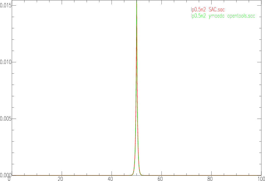
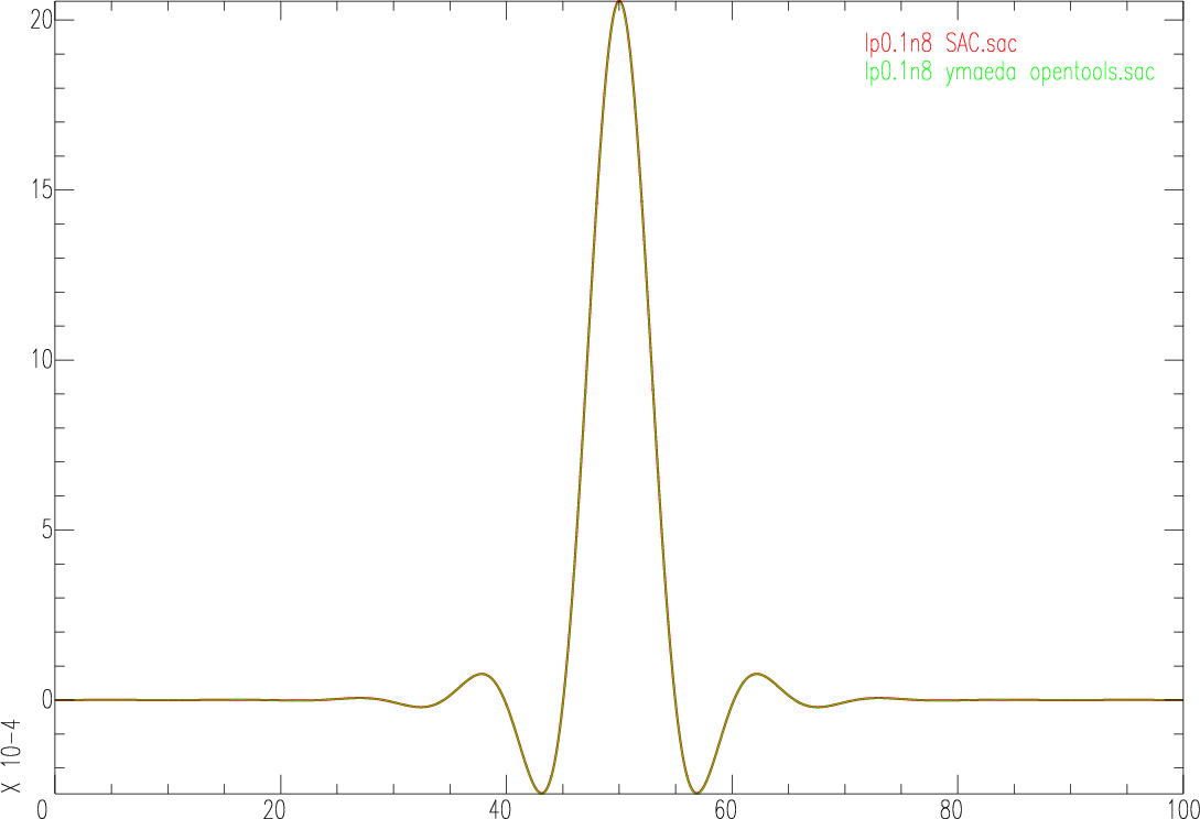
r input.sac
lp bu co 0.5 n 1 p 2
w lp0.5n2_SAC.sac

次にinput.sacに対してこの関数を用いて同じフィルターを掛け、結果をファイル(lp0.5n2_ymaeda_opentools.sac)に出力する。これには以下のC言語プログラムを作成・実行すれば良い。
Next, apply the same filter to input.sac using this function, and output the result to a file (filter_by_ymaeda_opentools). This step is realized by the C program shown below.

#include <inc.h>
int main(void)
{
  struct sac_timeseq raw,filtered;
  raw=read_sac_timeseq("input.sac");
  filtered.data=saito_butterworth_lp_zerophase(raw.data,0.5,2);
  filtered.header=copy_sac_header(raw.header);
  write_sac_timeseq("lp0.5n2_ymaeda_opentools.sac",filtered);
  return 0;
}

結果はSACの以下のコマンドにより比較できる。この例ではSACによるフィルタリングの結果を太い赤線、この関数によるフィルタリングの結果を細い緑線として重ねてプロットしている。
Results can be compared by SAC commands below. In this example, the two filtered waveforms are overlain using a thick red line for the filter by SAC and a thin green line for the filter by this function.

r lp0.5n2_SAC.sac lp0.5n2_ymaeda_opentools.sac
qdp off
color red increment on list red green
width list 3 1 increment
p2

比較の結果を下図に示す。 2つの結果は完全に一致していることが分かる。
The result of this comparison is shown below, indicating a complete match between the two results.

コーナー周波数を0.1 Hz、極の数を最小位相フィルター1回あたり4(合計8)とした場合の比較も下図に示す。この場合もSACによるフィルタリングとこの関数によるフィルタリングの結果は完全に一致している。
Results from a corner frequency of 0.1 Hz with four poles in each minimum phase filter (eight poles in total) are shown below. In this case also, the filtering results by SAC and this function are completely equal.